Abstract
Test-time prompt tuning (TPT) adapts CLIP’s text prompt to each test image by minimizing the entropy of predictions over augmented views. It raises zero-shot accuracy, but it also makes the model overconfident, so the expected calibration error (ECE) goes up a lot. C-TPT addressed this with an Average Text Feature Dispersion (ATFD) loss that pushes class text features away from their centroid in L2 distance. The authors argue that this is not enough. On the unit hypersphere, moving the centroid toward the origin does not guarantee that individual class features are far apart from each other. In hard cases some features still sit close together, and those cases have high ECE.
O-TPT replaces dispersion with an angular objective. It adds a penalty that pushes the matrix of pairwise cosine similarities between class text features toward the identity, so the features become close to orthogonal. The authors show that lower cosine similarity between text features goes with lower ECE, and that this simple constraint lowers ECE more than C-TPT and the Robust-Adapt variants.
Motivation
The starting point is an observation about hand-crafted prompts: different prompt styles can give CLIP almost the same accuracy but very different calibration. C-TPT explained this with L2 dispersion of text features around their centroid. The authors look at the angles instead. For several prompt styles on Caltech101 (zero-shot CLIP), they plot the distribution of pairwise cosine similarities between the class text features.
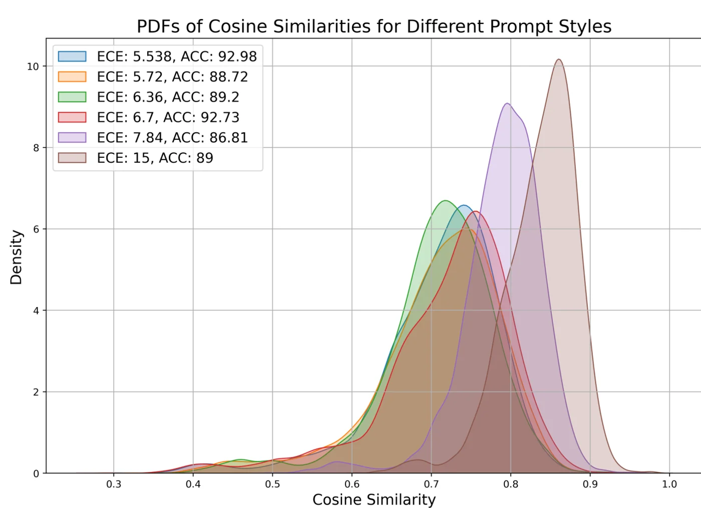 Distribution of pairwise cosine similarities between class text features on Caltech101, one curve per hand-crafted prompt style. Prompts with lower ECE sit further left (lower similarity, larger angles); the worst prompt (ECE 15) peaks near 0.86, even though its accuracy (89) is similar to the others. Figure from the paper.
The ordering is clean: the ECE 5.5-5.7 prompts peak around 0.72-0.74, the ECE 7.84 prompt near 0.80, and the ECE 15 prompt near 0.86. Accuracy does not follow this order at all. The appendix repeats the check with 80 prompt templates on seven datasets and finds the same relation between mean cosine similarity and ECE. So the angle between class features, not only their spread around a centroid, seems to carry the calibration signal.
The second piece of evidence is per test sample. On Flowers, the authors run TPT, C-TPT and O-TPT and record, for each test image, the mean cosine similarity of the tuned class text features.
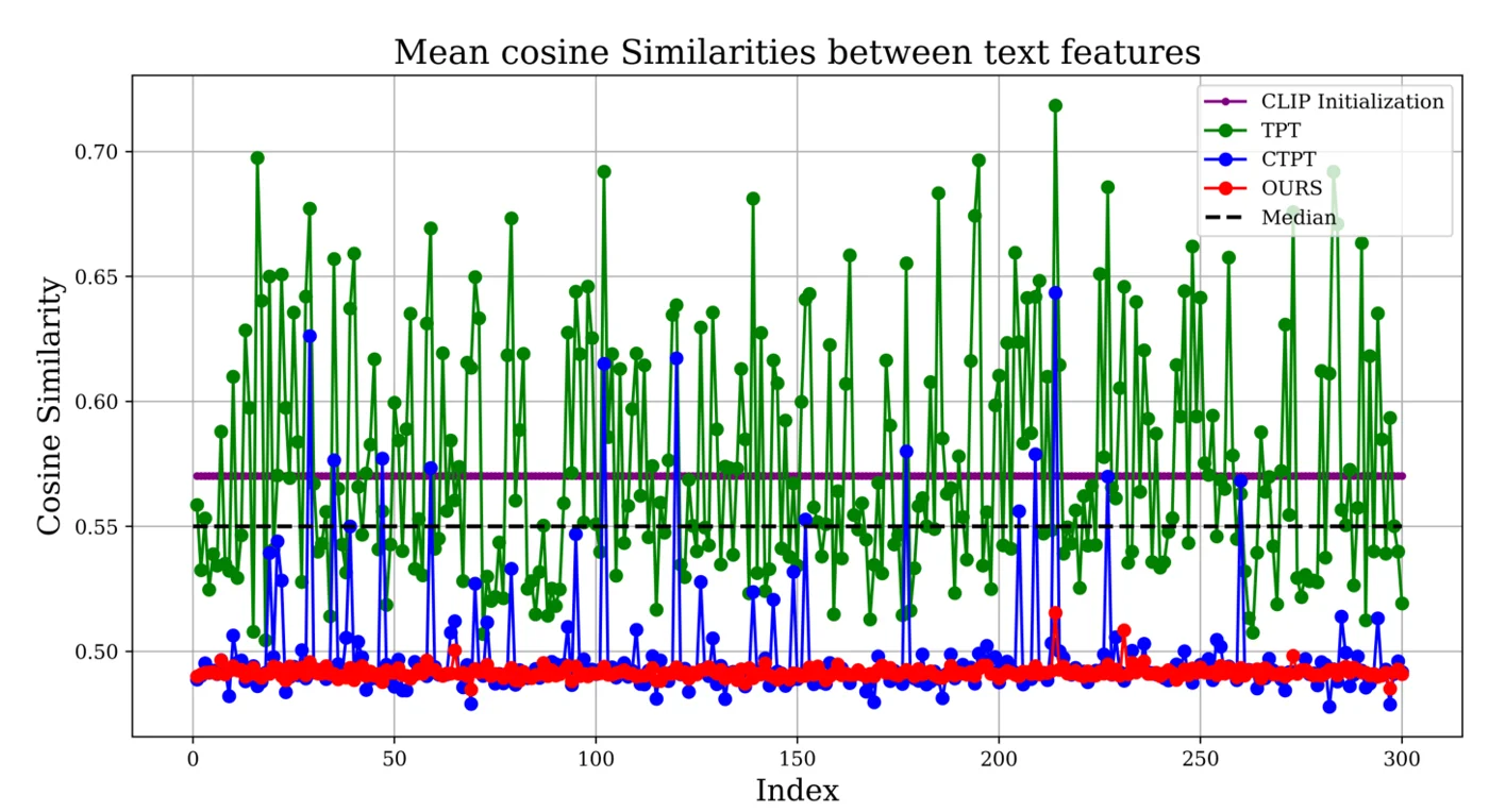 Mean pairwise cosine similarity of the tuned text features for each test sample on Flowers (CLIP ViT-B/16). TPT (green) pushes similarity above the CLIP initialization (purple) for many samples and fluctuates strongly. C-TPT (blue) mostly stays low but has frequent spikes back to 0.55-0.65. O-TPT (red) stays flat around 0.49. Figure from the paper.
TPT’s entropy minimization often pulls class features together, which is when it becomes overconfident. C-TPT fixes this for most samples, but its spikes land on the same hard samples where TPT fails, and these are exactly the samples with high ECE (Group 1 in the analysis below). The insight O-TPT builds on is that L2 dispersion can be satisfied by moving the centroid without separating every pair, so it is better to penalize pairwise angles directly.
Method
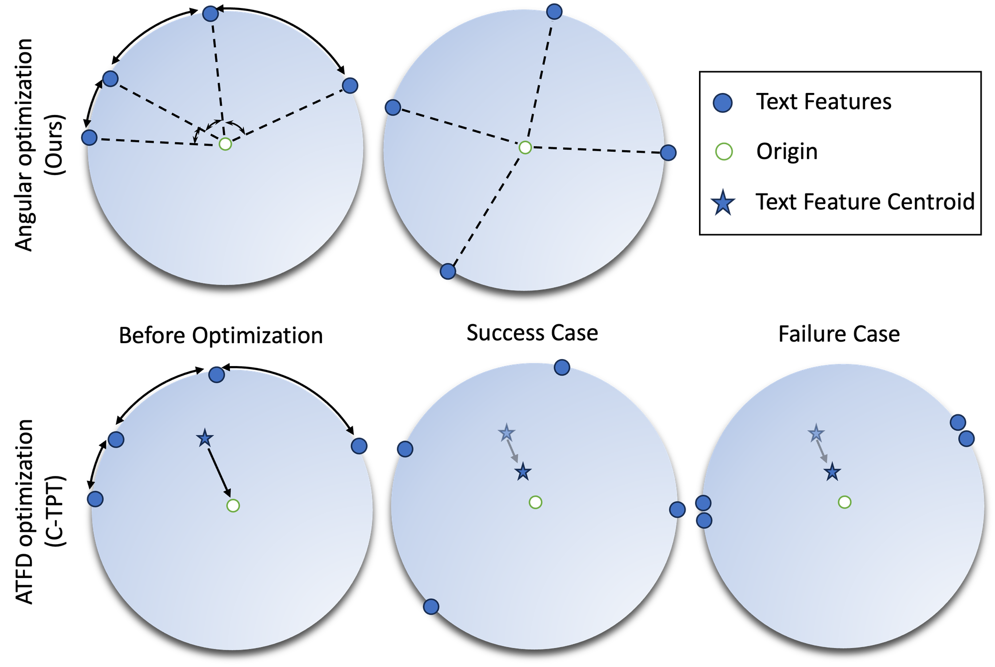 Angular optimization (O-TPT, top) versus ATFD optimization (C-TPT, bottom) on the hypersphere of text features. ATFD moves the centroid toward the origin, which can succeed or can still leave features clustered. O-TPT spreads the features by angle. Figure from the paper.
Setup
CLIP has a text encoder \(\mathbf{f}_T\) and an image encoder \(\mathbf{f}_I\). For each class \(c_i\) a prompt \(\mathbf{t}_{c_i}\) (e.g. “a photo of a {class}”) gives a text feature \(\mathbf{e}_{c_i} = \mathbf{f}_T(\mathbf{t}_{c_i})\). A test image gives \(\mathbf{v} = \mathbf{f}_I(I)\), and the class probabilities are a softmax over cosine similarities \(s_i = \cos(\mathbf{v}, \mathbf{e}_{c_i})\) with a temperature \(\tau\). In TPT the prompt tokens are learnable and are updated with one gradient step per test image, using the entropy loss \(L_{TPT}\) on confident augmented views. Calibration is measured with ECE:
\[\text{ECE} = \sum_{m=1}^{M} \frac{\lvert A_m \rvert}{N} \left\lvert \text{acc}(A_m) - \text{conf}(A_m) \right\rvert.\]Why angles and not L2 dispersion
The figure shows the argument. Normalized CLIP text features lie on the unit hypersphere. ATFD (bottom row) maximizes the distance of each feature from the centroid, which in practice moves the centroid toward the origin. In the success case this spreads the features. In the failure case the centroid moves but some pairs of features stay close together, so the space is underused.
The authors support this with two analyses. First, over many hand-crafted prompt styles, prompts with lower ECE have cosine similarity distributions shifted toward lower values. Second, they split test samples by whether TPT’s text features have above-median (Group 1) or below-median (Group 2) mean cosine similarity. On the harder Group 1, ECE is 15.97 for TPT, 6.04 for C-TPT, and 4.75 for O-TPT. So the samples where text features collapse are where calibration fails, and C-TPT does not fix them fully.
The orthogonality constraint
Stack the text features of all \(C\) classes into \(\mathbf{E} \in \mathbb{R}^{C\times D}\). Then \(\mathbf{E}\mathbf{E}^T\) holds the pairwise cosine similarities. The ideal is \(\mathbf{E}\mathbf{E}^T = I_C\), where all class features are orthogonal. O-TPT adds this as a penalty to the TPT loss:
\[\mathbf{t}^{*} = \arg\min_{\mathbf{t}} \left( L_{TPT} + \lambda \left\lVert \mathbf{E}\mathbf{E}^{T} - I_C \right\rVert_2^2 \right).\]Only the prompt \(\mathbf{t}\) is optimized. For normalized features the diagonal of \(\mathbf{E}\mathbf{E}^T\) is already 1, so in effect the term pushes every off-diagonal cosine similarity toward zero. That is what the top row of the figure shows: features spread out by angle instead of only moving the centroid.
Details
The prompt is initialized from a hard prompt, as in C-TPT, and updated with a single AdamW step (learning rate 0.005, batch of 64 augmented views). A Householder transform is applied on top of \(\mathbf{E}\mathbf{E}^T\) to help the one-step optimization. The paper does not describe this step in detail, but it reports that removing it raises the average ECE on the fine-grained benchmarks from 4.23 to 4.45 (ViT-B/16). The weight is \(\lambda = 18\) for fine-grained datasets and \(\lambda = 2\) for the ImageNet variants.
Main Experiments
Backbones are CLIP ViT-B/16 and CLIP RN50. Metrics are top-1 accuracy (%) and ECE (%). The fine-grained table shows only the Average column of the paper’s Tables 4 and 5, which averages 11 datasets (ImageNet, DTD, Flowers, Food101, SUN397, Aircraft, Pets, Caltech101, UCF101, EuroSAT, Cars). The Robust-Adapt rows are the logit-normalization methods of Murugesan et al. applied together with C-TPT.
Fine-grained classification, average over 11 datasets
| Method | ViT-B/16 Acc. | ViT-B/16 ECE | RN50 Acc. | RN50 ECE |
|---|---|---|---|---|
| Zero-shot CLIP | 63.7 | 4.43 | 55.9 | 5.61 |
| TPT | 65.0 | 11.6 | 57.7 | 11.7 |
| C-TPT | 64.57 | 5.13 | 57.75 | 6.19 |
| Robust-adapt-SaLs-CTPT | 64.55 | 5.69 | 57.20 | 6.82 |
| Robust-adapt-Penalty-CTPT | 64.65 | 4.66 | 57.40 | 6.41 |
| Robust-adapt-ZS-CTPT | 64.51 | 5.09 | 57.41 | 6.34 |
| O-TPT | 64.41 | 4.23 | 57.47 | 5.45 |
Natural distribution shifts, average over ImageNet-A, -V2, -R, -Sketch (Average column of Table 6)
| Method | ViT-B/16 Acc. | ViT-B/16 ECE | RN50 Acc. | RN50 ECE |
|---|---|---|---|---|
| Zero-shot CLIP | 57.2 | 5.04 | 40.6 | 7.46 |
| TPT | 59.9 | 12.0 | 43.5 | 16.7 |
| C-TPT | 59.6 | 5.82 | 42.8 | 12.1 |
| O-TPT | 57.80 | 4.88 | 41.16 | 9.69 |
O-TPT has the lowest average ECE among the test-time methods on both benchmarks and both backbones. On the fine-grained benchmarks its ECE is also below zero-shot CLIP, which no other test-time method in the table achieves. The text of the paper quotes 4.21 for the ViT-B/16 average ECE, while the table gives 4.23; the table value is used here. The calibration gain costs some accuracy: about 0.6 points versus TPT on fine-grained datasets with ViT-B/16, and 2.1 points on the ImageNet variants. O-TPT also lowers ECE when added on top of CoOp prompts (average ECE 7.91 vs. 10.04 for C-TPT and 18.36 for TPT) and on top of MaPLe.
The per-dataset picture is less uniform than the averages. The paper’s teaser compares ECE per dataset against C-TPT and the best Robust-Adapt variant.
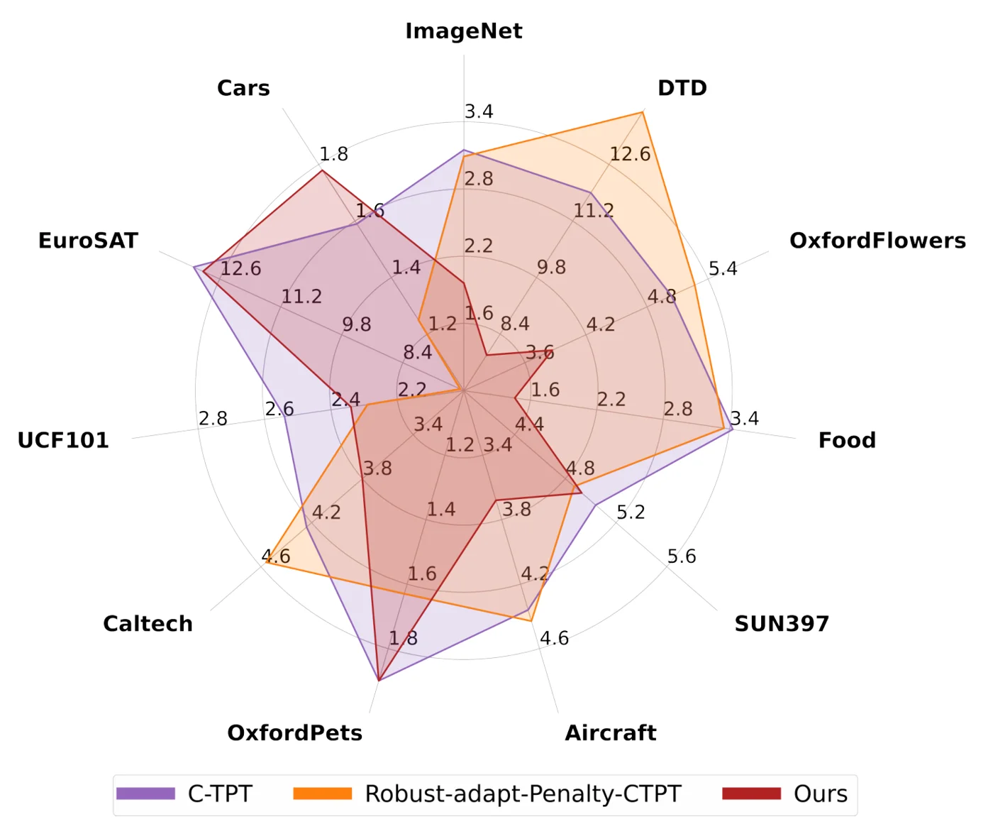 ECE per fine-grained dataset for C-TPT (purple), Robust-adapt-Penalty-CTPT (orange) and O-TPT (red); each axis has its own scale and smaller is better. O-TPT is much lower on DTD, Flowers, Food and Aircraft, but higher than the others on Cars and about level with C-TPT on EuroSAT and Pets. Figure from the paper.
The biggest gains come on DTD, Flowers and Food, where C-TPT is still clearly overconfident. On Cars O-TPT is the worst of the three, but all values there are below 2, so the absolute difference is small.
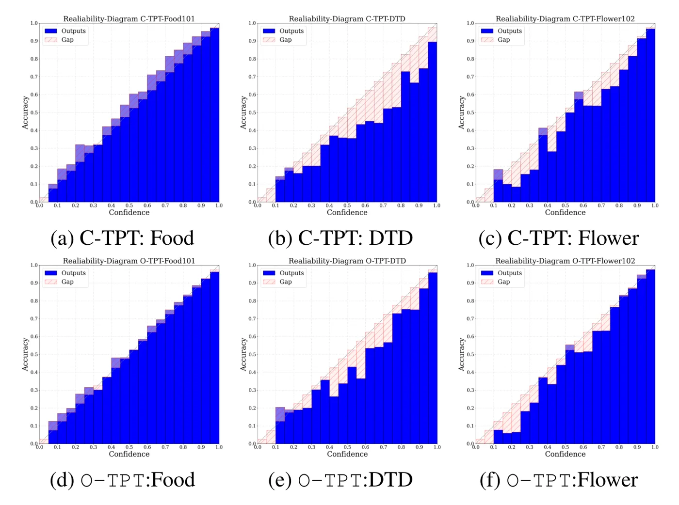 Reliability diagrams (CLIP ViT-B/16) for C-TPT (top) and O-TPT (bottom) on Food101, DTD and Flowers. Bars below the diagonal mean overconfidence, bars above it underconfidence. O-TPT shrinks the overconfident gaps on DTD and Flowers and removes C-TPT’s slight underconfidence on Food. Figure from the paper.
The reliability diagrams show that O-TPT does not just trade overconfidence for underconfidence: on Food the C-TPT bars sit above the diagonal and O-TPT moves them onto it, while on DTD and Flowers the large hatched gaps of C-TPT become smaller. DTD still has visible gaps at mid confidence.
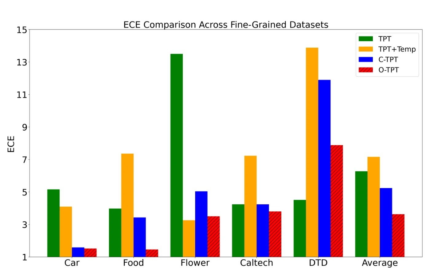 ECE of TPT, TPT with temperature scaling, C-TPT and O-TPT on five fine-grained datasets and their average. The temperature is fit on a separate labeled validation set, yet O-TPT has the lowest average ECE. Figure from the paper.
This comparison matters because temperature scaling uses labels that a test-time method does not have. In this plot TPT+Temp is even worse than plain TPT on average (it helps on Cars and Flowers but hurts on Food, Caltech and DTD), which suggests a single temperature learned on another split does not transfer well to per-sample prompt tuning.
Limitations
- No stated limitations. The paper does not have a limitations section.
- Accuracy drop on distribution shifts. On the ImageNet variants with ViT-B/16, accuracy falls from 59.9 (TPT) to 57.80, and ImageNet-R drops to 72.55, below zero-shot CLIP (74.0). Most of TPT’s accuracy gain is lost there.
- Not always better than zero-shot. With RN50 on natural shifts, O-TPT’s average ECE (9.69) is still above zero-shot CLIP (7.46).
- Exact orthogonality is impossible when classes outnumber dimensions. \(\mathbf{E}\mathbf{E}^T\) has rank at most \(D\), so with 1000 ImageNet classes and a 512-d ViT-B/16 embedding the target \(I_C\) cannot be reached. The penalty still lowers average similarity, but its optimum is no longer clear. The follow-up A-TPT builds on this point.
- Hyperparameter choice. \(\lambda\) is 18 for fine-grained data and 2 for ImageNet variants. How to set it for a new target domain without labels is not discussed. A Pareto plot over \(\lambda\) is given only for Food101 and Flowers.
- Cost. The penalty needs the full \(C\times C\) similarity matrix for every test image, which costs \(O(C^2 D)\) on top of TPT. The main paper does not report runtime or memory. The Householder step is described only briefly.
- Some datasets stay poorly calibrated. EuroSAT ECE is 12.98 with ViT-B/16 and 14.71 with RN50, almost unchanged from C-TPT.