Abstract
Point clouds at test time are often corrupted, for example by LiDAR sensor failures or by environmental factors. Most TTA methods fine-tune the source model with pseudo-labels or a self-supervised loss. Over a long test stream, these updates can accumulate errors and make the model forget useful source knowledge. In 2D, another line of work leaves the model alone and uses a diffusion model to move the test image back to the source domain. The authors say this had not been done for 3D point clouds, because point clouds are unstructured and hard to keep faithful during denoising.
3DD-TTA brings this input-adaptation idea to 3D. It uses LION, a latent diffusion model for point clouds. The test point cloud is encoded into a shape latent and a set of latent points. The latent points get a small amount of noise and are then denoised for a few DDIM steps. During denoising, a Selective Chamfer Distance keeps them close to the original. The cleaned latents are decoded and passed to the unchanged classifier. No network weights are updated.
Motivation
The authors start from a weakness shared by pseudo-label and self-supervised TTA on point clouds: every test sample changes the source weights. Early on this helps, but over a long stream the errors pile up and source knowledge is forgotten. Diffusion-based input adaptation (DDA and similar 2D work) avoids this by keeping the model fixed and moving the input instead. Nobody had made that work for point clouds, where there is no pixel grid and a denoiser can easily turn a corrupted chair into a clean but different chair.
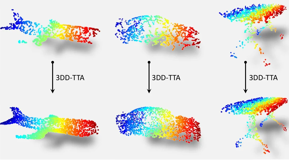 Corrupted test point clouds (top) and the same shapes after 3DD-TTA (bottom). Holes are filled and stray points are pulled back onto the surface, while the overall shape is kept. Figure from the paper.
The second observation is what makes one procedure work for many corruptions. Before perturbation, the Chamfer distance between a clean ShapeNet shape and its corrupted version has a very different distribution for uniform noise, Gaussian noise and RBF deformation. After a small amount of Gaussian noise is added to the latent points, the three distributions almost coincide. The noisy latent no longer carries a corruption-specific signature, so a single source denoiser can handle all of them without knowing which corruption it is seeing.
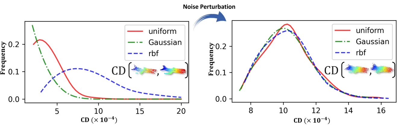 Distribution of the Chamfer distance between original and corrupted ShapeNet point clouds for three corruptions, before (left) and after (right) Gaussian perturbation of the latent points. After perturbation the curves overlap, which the authors read as corruption independence. Figure from the paper.
Method
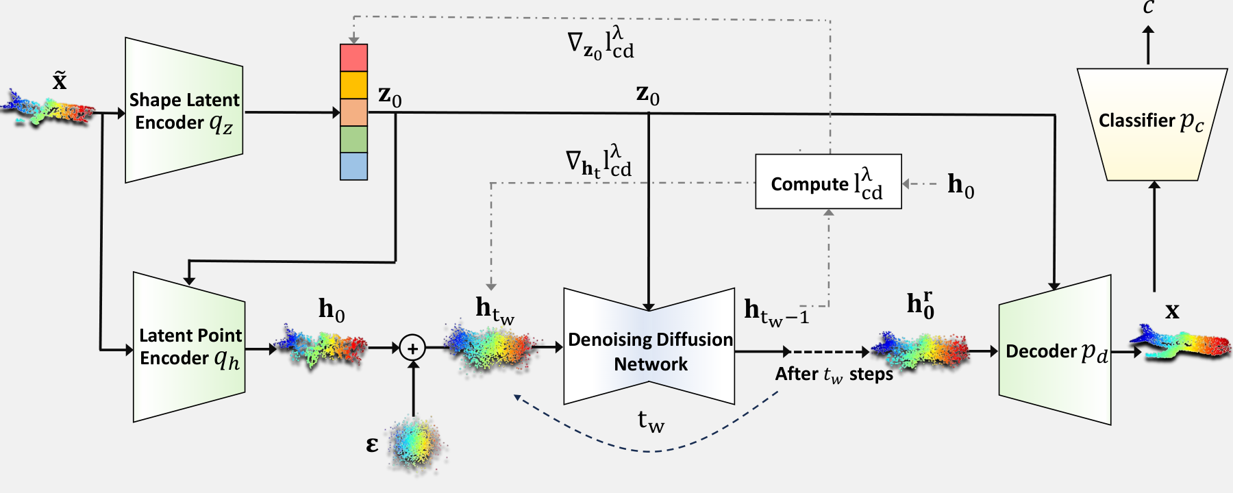 The corrupted input \(\tilde{\mathbf{x}}\) is encoded into a shape latent \(\mathbf{z}_0\) and latent points \(\mathbf{h}_0\). The latent points are noised to step \(t_w\), then denoised for \(t_w\) steps with SCD guidance on both \(\mathbf{h}_t\) and \(\mathbf{z}_0\). The result is decoded and classified by \(p_c\). Figure from the paper.
Backbone: LION
LION is a hierarchical VAE with a diffusion prior. It has two encoders:
- \(q_z(\mathbf{z}_0 \mid \mathbf{x})\) gives a global shape latent \(\mathbf{z}_0 \in \mathbb{R}^{D_z}\).
- \(q_h(\mathbf{h}_0 \mid \mathbf{z}_0, \mathbf{x})\) gives latent points \(\mathbf{h}_0 \in \mathbb{R}^{4 \times n}\). These are \(xyz\) coordinates plus one extra feature per point.
A denoiser \(\boldsymbol{\epsilon}_h(\mathbf{h}_t, \mathbf{z}_0, t)\) models the latent points conditioned on the shape latent. A decoder \(p_d(\mathbf{x} \mid \mathbf{z}_0, \mathbf{h}_0)\) maps the latents back to a point cloud. The whole model is pre-trained on ShapeNet, which is the source domain. The classifier \(p_c\) (Point-MAE) and the diffusion model both stay frozen.
Step 1: Encode and perturb (left half of the figure)
The corrupted input is encoded:
\[\mathbf{z}_0 \sim q_z(\mathbf{z}_0 \mid \tilde{\mathbf{x}}), \qquad \mathbf{h}_0 \sim q_h(\mathbf{h}_0 \mid \mathbf{z}_0, \tilde{\mathbf{x}})\]Then the latent points are noised forward to step \(t_w\):
\[\mathbf{h}_{t_w} = \sqrt{\bar\alpha_{t_w}}\, \mathbf{h}_0 + \sqrt{1 - \bar\alpha_{t_w}}\, \boldsymbol{\epsilon}\]The authors argue this noise makes the input less dependent on the specific corruption. Their Figure 2 shows that after perturbation, the Chamfer distance to the clean shape has nearly the same distribution for uniform noise, Gaussian noise and RBF corruption. The model therefore does not need to know which corruption it faces.
Step 2: Guided DDIM denoising (middle loop)
For \(t = t_w, \dots, 1\), the denoiser predicts the noise \(\boldsymbol{\epsilon}_t = \boldsymbol{\epsilon}_h(\mathbf{h}_t, \mathbf{z}_0, t)\). This gives an estimate of the clean latent points:
\[\bar{\mathbf{h}}_0 = \frac{\mathbf{h}_t - \sqrt{1 - \bar\alpha_t}\, \boldsymbol{\epsilon}_t}{\sqrt{\bar\alpha_t}}\]A deterministic DDIM step plus a guidance term then gives the next latent:
\[\mathbf{h}_{t-1} = \sqrt{\bar\alpha_{t-1}}\, \bar{\mathbf{h}}_0 + \sqrt{1 - \bar\alpha_{t-1}}\, \boldsymbol{\epsilon}_t - \eta \nabla_{\mathbf{h}_t} l^{\lambda}_{cd}\]Without guidance, the denoiser could drift to a different but plausible shape. The guidance keeps \(\bar{\mathbf{h}}_0\) close to the original latent points \(\mathbf{h}_0\).
Selective Chamfer Distance (SCD). The original \(\mathbf{h}_0\) is itself corrupted, so matching it exactly would bring the corruption back. SCD keeps only the closest \(\lambda\) fraction of nearest-neighbor distances in each direction and drops the rest as likely outliers:
\[l^{\lambda}_{cd}(\mathbf{h}_0, \bar{\mathbf{h}}_0) = \frac{1}{|\mathbf{h}_0|} \sum \mathrm{lower}_\lambda\big(\mathrm{sort}(D_{\mathbf{h}_0})\big) + \frac{1}{|\bar{\mathbf{h}}_0|} \sum \mathrm{lower}_\lambda\big(\mathrm{sort}(D_{\bar{\mathbf{h}}_0})\big)\]\(D_{\mathbf{h}_0}\) is the set of squared distances from each point in \(\mathbf{h}_0\) to its nearest point in \(\bar{\mathbf{h}}_0\). \(D_{\bar{\mathbf{h}}_0}\) is the same in the other direction. The paper uses \(\lambda = 0.96\).
Shape latent update. The shape latent from a corrupted input can give the denoiser poor conditioning. So it is also moved along the SCD gradient at every step (the top dashed arrow):
\[\mathbf{z}_0 \leftarrow \mathbf{z}_0 - \gamma \nabla_{\mathbf{z}_0} l^{\lambda}_{cd}\]Step 3: Decode and classify (right side)
After \(t_w\) steps, the rectified latent points \(\mathbf{h}_0^r\) and the updated \(\mathbf{z}_0\) are decoded into \(\mathbf{x}\). The frozen classifier then predicts \(c \sim p_c(c \mid \mathbf{x})\).
Settings: DDIM with 100 total steps, so each step skips 10 of LION’s 1000 training steps. The input is noised to step \(t_w = 5\) and denoised for 5 steps, with \(\gamma = \eta = 0.01\).
Main Experiments
The source classifier is Point-MAE as trained in MATE. The metric is the mean accuracy (%) over 15 corruptions. LION is pre-trained only on ShapeNet, so ModelNet40-c and ScanObjectNN-c also test cross-dataset generalization. ScanObjectNN-c was compared only against the source model.
| Method | ShapeNet-c | ModelNet40-c | ScanObjectNN-c |
|---|---|---|---|
| Point-MAE (src) | 59.3 | 57.6 | 61.5 |
| DUA | 60.8 | 54.7 | - |
| TTT-Rot | 60.9 | 53.0 | - |
| SHOT | 36.2 | 26.6 | - |
| T3A | 54.4 | 55.7 | - |
| TENT | 37.4 | 26.5 | - |
| MATE-S | 63.1 | 64.3 | - |
| 3DD-TTA | 69.8 | 65.7 | 64.3 |
Selected corruptions on ShapeNet-c (subset of Table 1, accuracy %):
| Method | gauss | back | impu | shear | rot | occ | Mean |
|---|---|---|---|---|---|---|---|
| Point-MAE (src) | 66.4 | 15.0 | 60.6 | 74.1 | 42.8 | 8.4 | 59.3 |
| DUA | 70.1 | 14.3 | 60.9 | 77.1 | 57.5 | 11.9 | 60.8 |
| MATE-S | 74.7 | 4.3 | 66.2 | 79.2 | 56.1 | 12.3 | 63.1 |
| 3DD-TTA | 80.7 | 77.6 | 77.2 | 77.2 | 50.4 | 14.9 | 69.8 |
Takeaways:
- The gains come mostly from noise corruptions. Background noise on ShapeNet-c goes from 15.0 to 77.6. The best baseline there, TTT-Rot, reaches only 23.1.
- Transformation corruptions are the weak spot. On ShapeNet-c, rotation (50.4) trails DUA and MATE-S. On ModelNet40-c, shear (63.7) and rotation (33.4) are close to or below the source model.
- Adaptation is fast. Five denoising steps take 40 ms per sample on an A6000 (Table 4), and the time grows linearly to 290 ms at 40 steps.
The qualitative examples show where the gains come from. Noise-type corruptions (uniform, background, impulse) and density changes (cut-out, density decrease) are turned back into clean, complete surfaces.
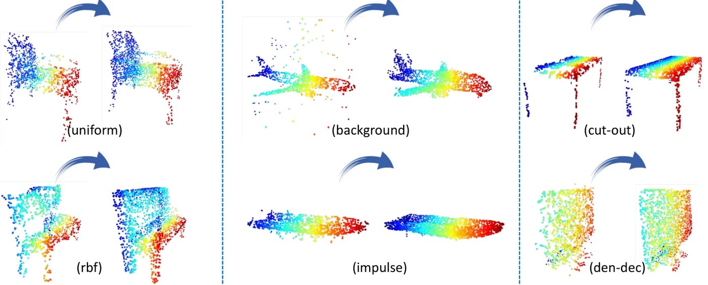 Corrupted inputs and their adapted versions for uniform, RBF, background, impulse, cut-out and density-decrease corruptions. Outliers are removed and missing parts are filled. Figure from the paper.
The step ablation explains the fixed setting of 5 denoising steps. Most corruptions peak at around 5 steps and slowly drop after that, while background noise keeps improving up to about 35 steps. Rotation stays near 0.5 regardless of the step count.
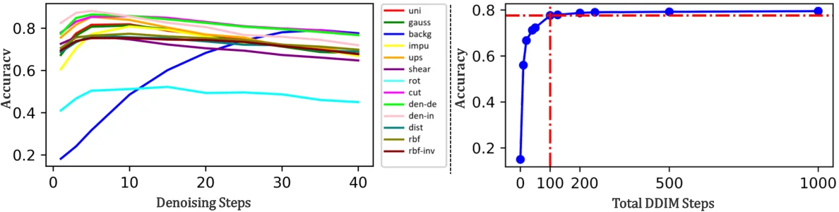 Left: accuracy per corruption as the number of denoising steps grows. Background noise (blue) is the only curve that needs many steps; rotation (cyan) barely moves. Right: with background noise, accuracy is stable down to about 100 total DDIM steps and collapses below that. Figure from the paper.
Limitations
- Rotation and shear (stated by the authors). A training-free denoiser cannot undo global geometric transformations well. On ModelNet40-c, shear drops below the source model (63.7 vs 67.6).
- Fixed step count (stated by the authors). Five steps work for most corruptions, but background noise needs up to 35, which takes longer. Choosing the number of steps per input is left to future work.
- A large pre-trained generative model is required. LION (a VAE plus latent diffusion priors) must be trained on the source domain. Here that is ShapeNet, and the same model is reused for the other datasets.
- Gradients through the denoiser. \(\bar{\mathbf{h}}_0\) depends on \(\mathbf{h}_t\) and \(\mathbf{z}_0\) through \(\boldsymbol{\epsilon}_h\). So both SCD updates need a backward pass through the denoising network at every step, not just forward passes.
- Limited baselines. The baselines are mostly 2D TTA methods plus MATE. There is no comparison with other diffusion-based input adaptation, such as a 3D port of DDA. On ScanObjectNN-c the only comparison is the source model.
- Occlusion and LiDAR stay hard. On ShapeNet-c, occlusion and LiDAR remain at 14.9 and 14.2.