Abstract
테스트 시점의 point cloud는 LiDAR 센서 고장이나 환경 요인 등으로 corruption이 생긴 경우가 많다. 대부분의 test-time adaptation (TTA) 방법은 pseudo-label이나 self-supervised loss로 source model을 fine-tuning한다. 테스트 스트림이 길어지면 이러한 update가 오류를 누적시키고, 모델이 유용한 source 지식을 잊게 만들 수 있다. 2D에서는 모델을 그대로 두고 diffusion model로 테스트 이미지를 source domain으로 되돌리는 또 다른 연구 흐름이 있다. 저자들은 3D point cloud에서는 이것이 시도된 적이 없다고 말한다. Point cloud는 비정형 데이터이고, denoising 과정에서 원본에 대한 fidelity를 유지하기 어렵기 때문이다.
3DD-TTA는 이러한 input adaptation 아이디어를 3D로 가져온다. Point cloud용 latent diffusion model인 LION을 사용한다. 테스트 point cloud는 shape latent와 latent point 집합으로 인코딩된다. Latent point에 소량의 noise를 더한 뒤 몇 step의 DDIM으로 denoising한다. Denoising 중에는 Selective Chamfer Distance가 latent point가 원본에서 멀어지지 않도록 붙잡아 둔다. 정제된 latent는 decoding되어 변경되지 않은 classifier에 입력된다. 어떤 네트워크 weight도 update되지 않는다.
Motivation
저자들의 출발점은 point cloud에서 pseudo-label 기반 TTA와 self-supervised TTA가 공통으로 가진 약점이다. 테스트 샘플마다 source weight가 바뀐다. 초반에는 도움이 되지만, 스트림이 길어지면 오류가 쌓이고 source 지식이 잊힌다. Diffusion 기반 input adaptation(DDA 등 2D 연구)은 모델을 고정하고 입력을 옮기는 방식으로 이를 피한다. 하지만 point cloud에서는 아무도 이를 성공시키지 못했다. Pixel grid가 없고, denoiser가 corruption이 있는 의자를 깨끗하지만 다른 의자로 바꿔 버리기 쉽기 때문이다.
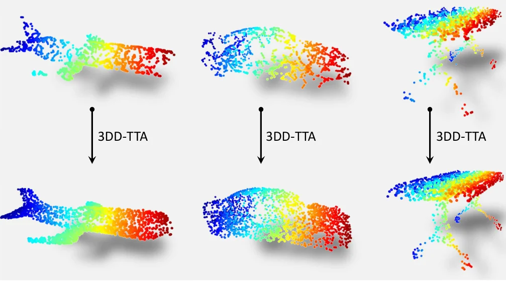 Corruption이 있는 테스트 point cloud(위)와 3DD-TTA 적용 후의 같은 형상(아래). 구멍은 채워지고 흩어진 점은 표면으로 돌아오며, 전체 형상은 유지된다. 논문 Figure.
두 번째 관찰은 하나의 절차가 여러 corruption에 통하는 이유를 설명한다. Perturbation 전에는 깨끗한 ShapeNet 형상과 corruption 버전 사이의 Chamfer distance 분포가 uniform noise, Gaussian noise, RBF deformation마다 크게 다르다. Latent point에 약간의 Gaussian noise를 더하면 세 분포가 거의 겹친다. Noise가 더해진 latent에는 corruption별 특징이 더 이상 남지 않으므로, source denoiser 하나가 어떤 corruption인지 모르는 채로 모두 처리할 수 있다.
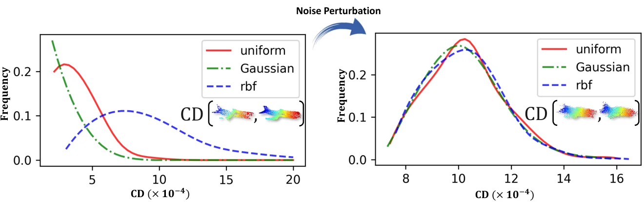 세 가지 corruption에 대해 원본과 corruption이 있는 ShapeNet point cloud 사이의 Chamfer distance 분포를 latent point의 Gaussian perturbation 전(왼쪽)과 후(오른쪽)로 나타냈다. Perturbation 후에는 곡선이 겹치며, 저자들은 이를 corruption independence로 해석한다. 논문 Figure.
Method
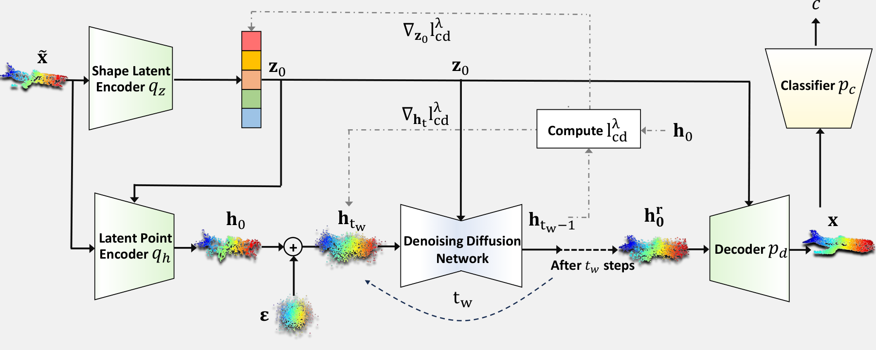 Corruption이 있는 입력 \(\tilde{\mathbf{x}}\)는 shape latent \(\mathbf{z}_0\)와 latent point \(\mathbf{h}_0\)로 인코딩된다. Latent point는 step \(t_w\)까지 noise가 더해진 뒤, \(\mathbf{h}_t\)와 \(\mathbf{z}_0\) 모두에 SCD guidance를 걸어 \(t_w\) step 동안 denoising된다. 결과는 decoding되어 \(p_c\)로 분류된다. 그림은 논문에서 가져왔다.
Backbone: LION
LION은 diffusion prior를 가진 hierarchical VAE이다. Encoder는 두 개다.
- \(q_z(\mathbf{z}_0 \mid \mathbf{x})\)는 global shape latent \(\mathbf{z}_0 \in \mathbb{R}^{D_z}\)를 만든다.
- \(q_h(\mathbf{h}_0 \mid \mathbf{z}_0, \mathbf{x})\)는 latent point \(\mathbf{h}_0 \in \mathbb{R}^{4 \times n}\)를 만든다. 이는 점마다 \(xyz\) 좌표와 추가 feature 하나로 이루어진다.
Denoiser \(\boldsymbol{\epsilon}_h(\mathbf{h}_t, \mathbf{z}_0, t)\)는 shape latent를 condition으로 latent point를 모델링한다. Decoder \(p_d(\mathbf{x} \mid \mathbf{z}_0, \mathbf{h}_0)\)는 latent를 다시 point cloud로 변환한다. 전체 모델은 source domain인 ShapeNet에서 pre-training된다. Classifier \(p_c\)(Point-MAE)와 diffusion model은 모두 고정된다.
Step 1: Encode and perturb (그림의 왼쪽 절반)
Corruption이 있는 입력을 인코딩한다.
\[\mathbf{z}_0 \sim q_z(\mathbf{z}_0 \mid \tilde{\mathbf{x}}), \qquad \mathbf{h}_0 \sim q_h(\mathbf{h}_0 \mid \mathbf{z}_0, \tilde{\mathbf{x}})\]그다음 latent point에 forward process로 step \(t_w\)까지 noise를 더한다.
\[\mathbf{h}_{t_w} = \sqrt{\bar\alpha_{t_w}}\, \mathbf{h}_0 + \sqrt{1 - \bar\alpha_{t_w}}\, \boldsymbol{\epsilon}\]저자들은 이 noise가 입력의 특정 corruption 유형에 대한 의존성을 줄인다고 주장한다. 논문의 Figure 2는 perturbation 이후 깨끗한 형상까지의 Chamfer distance가 uniform noise, Gaussian noise, RBF corruption에서 거의 같은 분포를 보임을 보여 준다. 따라서 모델은 자신이 어떤 corruption을 마주했는지 알 필요가 없다.
Step 2: Guided DDIM denoising (가운데 루프)
\(t = t_w, \dots, 1\)에 대해 denoiser는 noise \(\boldsymbol{\epsilon}_t = \boldsymbol{\epsilon}_h(\mathbf{h}_t, \mathbf{z}_0, t)\)를 예측한다. 이로부터 깨끗한 latent point의 추정치를 얻는다.
\[\bar{\mathbf{h}}_0 = \frac{\mathbf{h}_t - \sqrt{1 - \bar\alpha_t}\, \boldsymbol{\epsilon}_t}{\sqrt{\bar\alpha_t}}\]Deterministic DDIM step에 guidance 항을 더해 다음 latent를 얻는다.
\[\mathbf{h}_{t-1} = \sqrt{\bar\alpha_{t-1}}\, \bar{\mathbf{h}}_0 + \sqrt{1 - \bar\alpha_{t-1}}\, \boldsymbol{\epsilon}_t - \eta \nabla_{\mathbf{h}_t} l^{\lambda}_{cd}\]Guidance가 없으면 denoiser는 그럴듯하지만 다른 형상으로 흘러갈 수 있다. Guidance는 \(\bar{\mathbf{h}}_0\)를 원래 latent point \(\mathbf{h}_0\)에 가깝게 유지한다.
Selective Chamfer Distance (SCD). 원래의 \(\mathbf{h}_0\) 자체에 corruption이 있으므로, 이를 정확히 맞추면 corruption이 다시 들어온다. SCD는 각 방향에서 nearest-neighbor distance 중 가장 가까운 \(\lambda\) 비율만 남기고, 나머지는 outlier일 가능성이 높다고 보고 버린다.
\[l^{\lambda}_{cd}(\mathbf{h}_0, \bar{\mathbf{h}}_0) = \frac{1}{|\mathbf{h}_0|} \sum \mathrm{lower}_\lambda\big(\mathrm{sort}(D_{\mathbf{h}_0})\big) + \frac{1}{|\bar{\mathbf{h}}_0|} \sum \mathrm{lower}_\lambda\big(\mathrm{sort}(D_{\bar{\mathbf{h}}_0})\big)\]\(D_{\mathbf{h}_0}\)는 \(\mathbf{h}_0\)의 각 점에서 \(\bar{\mathbf{h}}_0\)의 가장 가까운 점까지의 squared distance 집합이다. \(D_{\bar{\mathbf{h}}_0}\)는 반대 방향으로 같은 것을 구한 것이다. 논문은 \(\lambda = 0.96\)을 사용한다.
Shape latent update. Corruption이 있는 입력에서 얻은 shape latent는 denoiser에 부적절한 condition을 줄 수 있다. 그래서 shape latent도 매 step SCD gradient 방향으로 이동시킨다(위쪽 점선 화살표).
\[\mathbf{z}_0 \leftarrow \mathbf{z}_0 - \gamma \nabla_{\mathbf{z}_0} l^{\lambda}_{cd}\]Step 3: Decode and classify (오른쪽)
\(t_w\) step이 끝나면 보정된 latent point \(\mathbf{h}_0^r\)와 update된 \(\mathbf{z}_0\)를 \(\mathbf{x}\)로 decoding한다. 그다음 고정된 classifier가 \(c \sim p_c(c \mid \mathbf{x})\)를 예측한다.
설정: 전체 100 step의 DDIM을 사용하므로 각 step은 LION의 1000개 training step 중 10개를 건너뛴다. 입력에는 step \(t_w = 5\)까지 noise를 더하고 5 step 동안 denoising하며, \(\gamma = \eta = 0.01\)이다.
Main Experiments
Source classifier는 MATE에서 학습한 Point-MAE이다. 평가 지표는 15가지 corruption에 대한 평균 accuracy(%)이다. LION은 ShapeNet에서만 pre-training되었으므로, ModelNet40-c와 ScanObjectNN-c는 cross-dataset generalization도 함께 시험한다. ScanObjectNN-c에서는 source model과만 비교했다.
| Method | ShapeNet-c | ModelNet40-c | ScanObjectNN-c |
|---|---|---|---|
| Point-MAE (src) | 59.3 | 57.6 | 61.5 |
| DUA | 60.8 | 54.7 | - |
| TTT-Rot | 60.9 | 53.0 | - |
| SHOT | 36.2 | 26.6 | - |
| T3A | 54.4 | 55.7 | - |
| TENT | 37.4 | 26.5 | - |
| MATE-S | 63.1 | 64.3 | - |
| 3DD-TTA | 69.8 | 65.7 | 64.3 |
ShapeNet-c의 일부 corruption 유형 (Table 1의 일부, accuracy %):
| Method | gauss | back | impu | shear | rot | occ | Avg |
|---|---|---|---|---|---|---|---|
| Point-MAE (src) | 66.4 | 15.0 | 60.6 | 74.1 | 42.8 | 8.4 | 59.3 |
| DUA | 70.1 | 14.3 | 60.9 | 77.1 | 57.5 | 11.9 | 60.8 |
| MATE-S | 74.7 | 4.3 | 66.2 | 79.2 | 56.1 | 12.3 | 63.1 |
| 3DD-TTA | 80.7 | 77.6 | 77.2 | 77.2 | 50.4 | 14.9 | 69.8 |
정리:
- 성능 향상은 주로 noise 계열 corruption에서 나온다. ShapeNet-c의 background noise는 15.0에서 77.6으로 오른다. 이 항목에서 가장 좋은 baseline인 TTT-Rot도 23.1에 그친다.
- Transformation 계열 corruption이 약점이다. ShapeNet-c에서 rotation(50.4)은 DUA와 MATE-S에 뒤진다. ModelNet40-c에서 shear(63.7)와 rotation(33.4)은 source model과 비슷하거나 그보다 낮다.
- Adaptation이 빠르다. 5 step denoising은 A6000에서 샘플당 40 ms가 걸리고(Table 4), 시간은 step 수에 비례해 40 step에서 290 ms까지 늘어난다.
Qualitative 예시를 보면 성능 향상이 어디서 오는지 알 수 있다. Noise 계열 corruption(uniform, background, impulse)과 density 변화(cut-out, density decrease)가 깨끗하고 완전한 표면으로 되돌아온다.
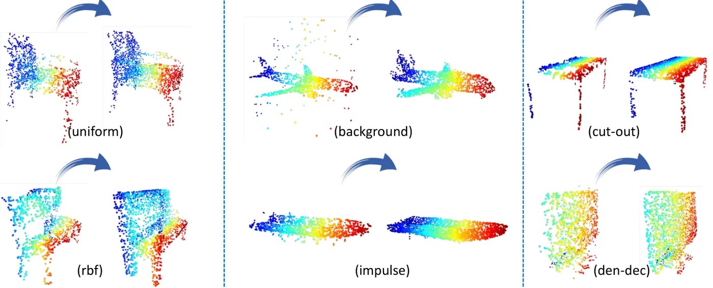 Uniform, RBF, background, impulse, cut-out, density-decrease corruption에 대한 입력과 adaptation 결과. Outlier는 제거되고 빠진 부분은 채워진다. 논문 Figure.
Step ablation은 denoising step을 5로 고정한 이유를 보여 준다. 대부분의 corruption은 5 step 부근에서 최고점을 찍고 그 뒤로 서서히 떨어지지만, background noise는 약 35 step까지 계속 좋아진다. Rotation은 step 수와 관계없이 0.5 근처에 머문다.
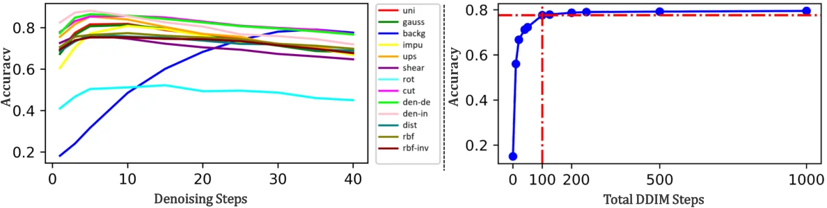 왼쪽: denoising step 수에 따른 corruption별 accuracy. 많은 step이 필요한 것은 background noise(파란색)뿐이고, rotation(하늘색)은 거의 움직이지 않는다. 오른쪽: background noise에서 accuracy는 전체 DDIM step 약 100까지는 안정적이고 그보다 적으면 급락한다. 논문 Figure.
Limitations
- Rotation과 shear (저자들이 직접 언급). 학습이 필요 없는 denoiser는 global geometric transformation을 잘 되돌리지 못한다. ModelNet40-c에서 shear는 source model보다 낮아진다(63.7 vs 67.6).
- 고정된 step 수 (저자들이 직접 언급). 대부분의 corruption에는 5 step이면 충분하지만, background noise는 최대 35 step이 필요해 시간이 더 걸린다. 입력마다 step 수를 정하는 문제는 향후 과제로 남겨 두었다.
- 대규모 pre-trained generative model이 필요하다. LION(VAE와 latent diffusion prior)을 source domain에서 학습해야 한다. 여기서는 ShapeNet이며, 같은 모델을 다른 데이터셋에도 재사용한다.
- Denoiser를 통한 gradient. \(\bar{\mathbf{h}}_0\)는 \(\boldsymbol{\epsilon}_h\)를 통해 \(\mathbf{h}_t\)와 \(\mathbf{z}_0\)에 의존한다. 따라서 두 SCD update 모두 매 step forward pass뿐 아니라 denoising network를 통한 backpropagation이 필요하다.
- 제한적인 baseline. Baseline은 대부분 2D TTA 방법과 MATE이다. DDA를 3D로 옮긴 것과 같은 다른 diffusion 기반 input adaptation 방법과의 비교는 없다. ScanObjectNN-c에서는 source model과의 비교만 있다.
- Occlusion과 LiDAR는 여전히 어렵다. ShapeNet-c에서 occlusion과 LiDAR는 각각 14.9와 14.2에 머문다.