Abstract
Test-time prompt tuning (TPT) adapts CLIP’s prompt to each unlabeled test image by entropy minimization. It improves accuracy but makes predictions overconfident. Two earlier fixes add a regularizer on the class text features. C-TPT pushes features away from their centroid in L2 distance (ATFD). O-TPT pushes the matrix of pairwise cosine similarities toward the identity, so features become orthogonal. The authors argue that neither guarantees an even spread of features on the hypersphere. ATFD can move the centroid while some features stay clustered. Orthogonality cannot be reached when the number of classes \(N\) is larger than the embedding dimension \(\lvert D \rvert\) (for example 1000 ImageNet classes in CLIP ViT-B/16’s 512-d space), and even when \(N < \lvert D \rvert\) it does not make the angles uniform.
A-TPT borrows the idea of the Tammes problem: place points on a sphere so that the minimum distance between any two is as large as possible. It adds a loss that maximizes, for each class, the angle to its closest other class feature. This spreads features uniformly in both the \(N > \lvert D \rvert\) and \(N < \lvert D \rvert\) regimes, and it lowers ECE further than C-TPT and O-TPT at a similar cost.
Motivation
The paper’s starting question is why prompts with almost the same accuracy can have very different calibration. Following C-TPT, the authors take 80 hard prompt templates for CLIP RN50 on Caltech101 and compare prompts within the same accuracy band. The ones with low ECE are also the ones whose class text features are spread out. In the t-SNE plot below, the poorly calibrated template “the nearest shape in this image is [class]” (ECE 10.84) collapses into a tight blob in the middle, regardless of class, while the well-calibrated templates sit next to their class clusters. Plain TPT produces the same kind of central blob. Adding A-TPT with growing \(\lambda\) breaks it up, and AD rises to 0.659 while ECE drops from 6.18 to 2.12.
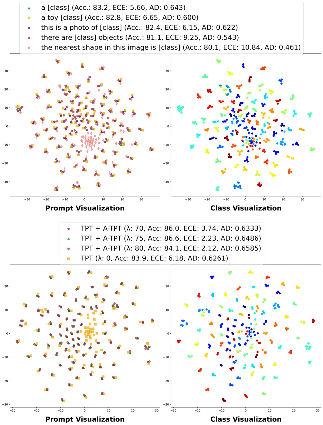 t-SNE of class text features from CLIP RN50 on Caltech101. Top: hard prompts; bottom: TPT and TPT + A-TPT. Left panels color by prompt, right panels by class. Low-AD prompts (pink diamonds on top, orange squares for TPT below) bunch up in the center, and those are the ones with high ECE. Figure from the paper.
The second observation is about O-TPT. Pushing cosines to zero sounds like the same goal, but it is not. On ImageNet-V2 (1000 classes, more than CLIP ViT-B/16’s 512 dimensions) the mean pairwise cosine under O-TPT jumps around from sample to sample, because exact orthogonality is impossible and the optimizer lands somewhere different each time. On EuroSAT (10 classes, fewer than 512) O-TPT settles at a mean cosine of about 0.77, while A-TPT reaches about 0.69, a wider spread than orthogonality alone produces in practice. This is why the authors switch from “make pairs orthogonal” to “make the closest pair as far apart as possible”.
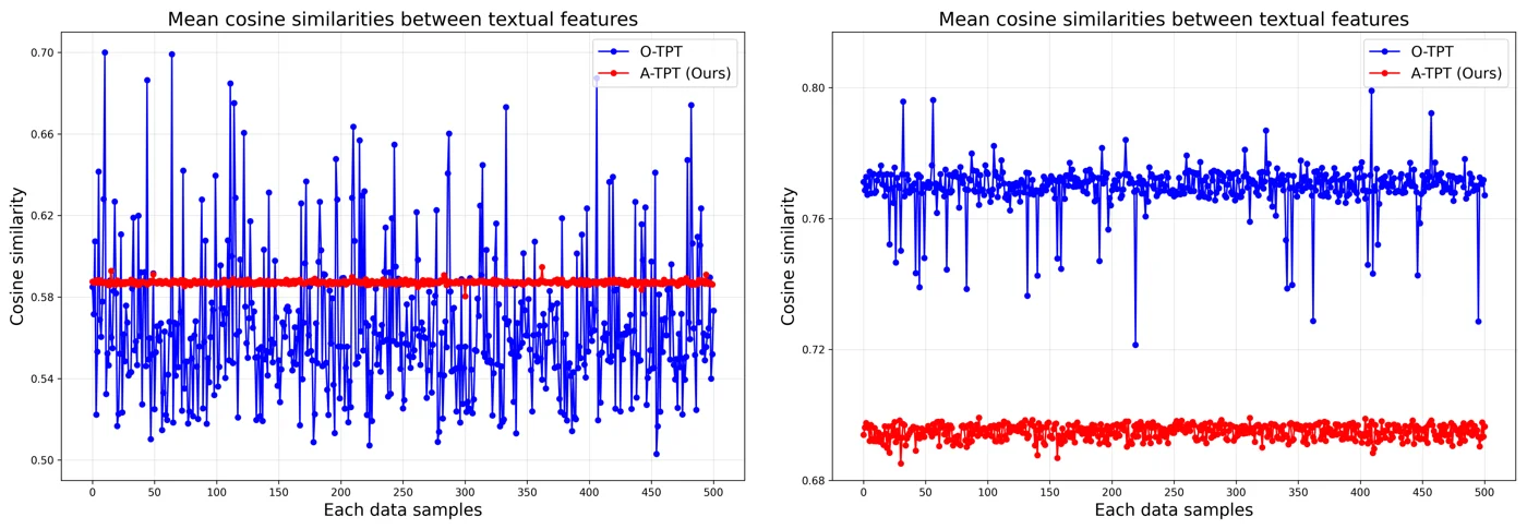 Mean cosine similarity between class text features for each test sample with CLIP ViT-B/16. Left: \(N > \lvert D \rvert\) (ImageNet-V2), where O-TPT (blue) fluctuates widely and A-TPT (red) stays flat. Right: \(N < \lvert D \rvert\) (EuroSAT), where A-TPT keeps features consistently further apart. Figure from the paper.
Method
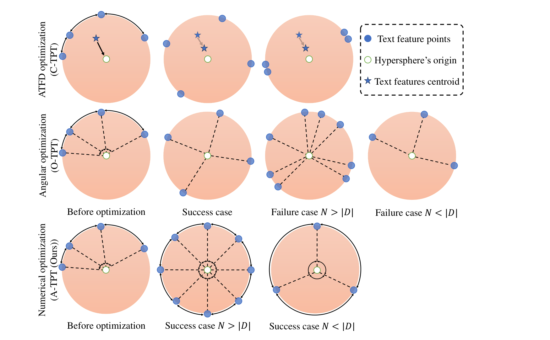 How ATFD (C-TPT, top), orthogonality (O-TPT, middle), and angular diversity (A-TPT, bottom) move class text features on the unit hypersphere. O-TPT fails in different ways when \(N > \lvert D \rvert\) and \(N < \lvert D \rvert\). A-TPT spreads the features evenly in both cases. Figure from the paper.
Setup
CLIP turns each class prompt \(\mathtt{p}_k\) into a text feature \(t_k = f_t(\mathtt{p}_k)\) and a test image into \(v = f_i(x)\). Class probabilities are a softmax over cosine similarities \(\text{sim}(v, t_k)\) with temperature 0.01. In TPT, the prompt tokens \(\mathtt{p}\) are learnable and get one gradient step per test image on the entropy loss \(\mathcal{L}_{\text{TPT}}\). The question is which extra term on the text features gives good calibration.
What goes wrong with dispersion and orthogonality
The top row of the figure is C-TPT. ATFD maximizes the L2 distance of features from their centroid. The centroid moves toward the origin, but in the failure case two features still sit next to each other.
The middle row is O-TPT. Its loss pushes all pairwise cosines to zero. When \(N > \lvert D \rvert\), \(N\) mutually orthogonal vectors do not exist, and the authors observe that features end up grouped closer together. When \(N < \lvert D \rvert\), orthogonality is reachable, but orthogonal features do not use the sphere as evenly as possible (three classes at 90 degrees from each other, instead of spread as far apart as possible).
The authors also argue from gradients. For O-TPT the gradient of a pairwise cosine with respect to a feature has norm
\[\left\lVert \frac{\partial \, Cos_{ij}}{\partial \mathbf{e}_i} \right\rVert = \frac{\lvert \sin\theta_{ij} \rvert}{\lVert \mathbf{e}_i \rVert},\]which goes to zero as \(\theta_{ij} \to 0\). So exactly the pairs that are nearly collinear, which hurt calibration most, get almost no push apart. Optimizing the angle itself gives
\[\left\lVert \frac{\partial \theta_{ij}}{\partial \mathbf{e}_i} \right\rVert = \frac{1}{\sin\theta_{ij}} \cdot \frac{\sin\theta_{ij}}{\lVert \mathbf{e}_i \rVert} = \frac{1}{\lVert \mathbf{e}_i \rVert},\]which does not depend on the angle.
Angular diversity loss
Stack the class text features into \(\mathbf{E} \in \mathbb{R}^{N\times \lvert D \rvert}\) and L2-normalize each row to get \(\hat{\mathbf{E}}\). The pairwise cosines and angles are
\[Cos = \hat{\mathbf{E}}\hat{\mathbf{E}}^T, \qquad \theta = \arccos(Cos).\]The angular diversity (AD) is the mean, over classes, of the angle to the nearest other class:
\[\text{AD} = \frac{1}{N} \sum_{i=1}^{N} \min_{j \neq i} \theta_{ij}.\]The prompt is tuned with
\[\mathtt{p}^{*} = \arg\min_{\mathtt{p}} \left( \mathcal{L}_{\text{TPT}} + \lambda \cdot \mathcal{L}_{\text{A-TPT}} \right), \qquad \mathcal{L}_{\text{A-TPT}} = -\text{AD}.\]Because only the nearest neighbour of each class counts, the loss targets the worst-separated pairs, which is the max-min idea of the Tammes problem. This is the bottom row of the figure: with \(N > \lvert D \rvert\) the features spread around the sphere at equal angles, and with \(N < \lvert D \rvert\) three features end up at equal, maximal angles rather than at 90 degrees.
Evidence and details
On Caltech101 with RN50, hard prompts with similar accuracy differ in ECE, and the better-calibrated ones have larger AD (for example “this is a photo of [class]”: ECE 6.15, AD 0.622; “the nearest shape in this image is [class]”: ECE 10.84, AD 0.461). With A-TPT added to TPT, the three reported prompts reach AD between 0.633 and 0.659 and ECE between 2.12 and 3.74, compared with AD 0.622 and ECE 6.18 for plain TPT. Implementation follows C-TPT and TPT: hard-prompt initialization, a single AdamW step with learning rate 5e-3, and batch size 64. The weight is \(\lambda = 80\) for fine-grained datasets and \(\lambda = 10\) for the ImageNet variants. The asymptotic cost is \(O(N^2 \lvert D \rvert)\), the same as O-TPT.
Main Experiments
Backbones are CLIP ViT-B/16 (512-d) and CLIP RN50 (1024-d). Metrics are top-1 accuracy (%) and ECE (%). The tables show only the Average column. The fine-grained average covers 11 datasets (ImageNet, DTD, Flowers102, Food101, SUN397, Aircraft, OxfordPets, Caltech101, UCF101, EuroSAT, StanfordCars). “Zero-shot” is the paper’s “Baseline” row. The C-TPT and O-TPT numbers are the same as those reported in the O-TPT paper.
Fine-grained classification, average over 11 datasets (Table 2)
| Method | ViT-B/16 Acc. | ViT-B/16 ECE | RN50 Acc. | RN50 ECE |
|---|---|---|---|---|
| Zero-shot CLIP | 63.70 | 4.43 | 55.90 | 5.61 |
| TPT | 65.00 | 11.60 | 57.70 | 11.70 |
| C-TPT | 64.57 | 5.13 | 57.75 | 6.19 |
| O-TPT | 64.41 | 4.23 | 57.47 | 5.45 |
| A-TPT | 64.92 | 2.61 | 57.53 | 2.92 |
Natural distribution shifts, average over ImageNet-A, -V2, -R, -Sketch (Table 3)
| Method | ViT-B/16 Acc. | ViT-B/16 ECE | RN50 Acc. | RN50 ECE |
|---|---|---|---|---|
| Zero-shot CLIP | 57.20 | 5.04 | 40.60 | 7.46 |
| TPT | 59.90 | 12.00 | 43.50 | 16.70 |
| C-TPT | 59.60 | 5.82 | 42.80 | 12.10 |
| O-TPT | 57.80 | 4.88 | 41.16 | 9.69 |
| A-TPT | 58.06 | 3.92 | 40.57 | 7.82 |
A-TPT has the lowest average ECE of the test-time methods in all four settings, and with ViT-B/16 on fine-grained data it keeps almost all of TPT’s accuracy (64.92 vs. 65.00). Its ECE is lower than O-TPT on every one of the 11 fine-grained datasets with both backbones, but a large part of the average gain comes from two datasets: EuroSAT, where ECE drops from 12.98 (O-TPT) to 3.92 with ViT-B/16 and from 14.71 to 2.51 with RN50, and DTD, where it drops from 7.88 to 4.76 and from 16.53 to 6.41. The paper’s text quotes 2.92 (ViT-B/16) and 2.79 (RN50) for the fine-grained average ECE, while Table 2 gives 2.61 and 2.92; the table values are used here. On ImageNet-V2 the extra cost over C-TPT is small: 1.058 s per batch and 21840 MiB, versus 1.055 s and 21838 MiB for C-TPT and 1.064 s and 23740 MiB for O-TPT.
The per-dataset bars make the concentration of the gain visible. A-TPT’s bar is the lowest almost everywhere, but the big gaps are at DTD and EuroSAT. On most other datasets the three methods are within one or two points.
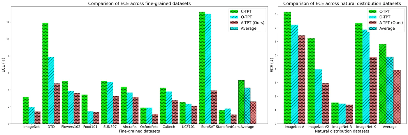 ECE per dataset with CLIP ViT-B/16 for fine-grained datasets (left) and natural distribution shifts (right). A-TPT (red) is lowest on nearly every dataset; the largest margins are on DTD, EuroSAT and ImageNet-K. Figure from the paper.
The reliability diagrams show the same thing at the level of individual bins. On DTD, C-TPT and O-TPT leave large gaps above the bars at medium and high confidence, meaning the model is more confident than it is accurate. A-TPT closes most of that gap, although some overconfidence remains around confidence 0.7 to 0.8.
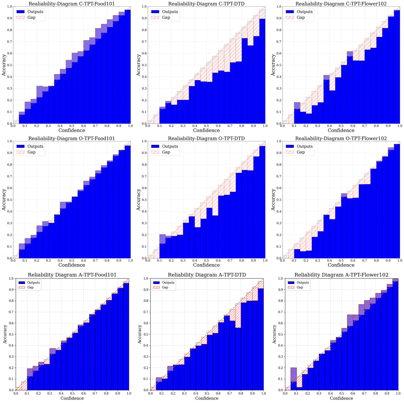 Reliability diagrams on Food101, DTD and Flowers102 with CLIP ViT-B/16. Rows: C-TPT, O-TPT, A-TPT. Hatched red areas are the gap to perfect calibration; they shrink most visibly for A-TPT on DTD and Flowers102. Figure from the paper (assembled from its panels).
Limitations
- Small accuracy drops (stated by the authors). Some datasets lose accuracy, which the authors put at under 1-2%. On natural shifts with RN50, A-TPT’s average accuracy (40.57) falls to the zero-shot level (40.60), so TPT’s accuracy gain is gone there.
- Fixed \(\lambda\) without labels (stated by the authors). The trade-off is set by one weight, which they fix from ablations and say may not be optimal per sample. In practice it is also changed per benchmark (80 for fine-grained data, 10 for ImageNet variants), which needs some knowledge of the target setting.
- Not always better than zero-shot. The paper says A-TPT beats zero-shot calibration on natural shifts on both backbones, but with RN50 its average ECE (7.82) is above zero-shot CLIP (7.46).
- Average gains are concentrated. EuroSAT and DTD drive much of the average ECE gap to O-TPT. On the other nine datasets the gains are consistent but smaller, about 0.1 to 2 ECE points.
- Hard minimum in the loss. Each class only gets a gradient through its single nearest neighbour, and \(\arccos\) has unbounded slope near cosine values of \(\pm 1\). The paper does not discuss stability issues from either, though results across seeds are reported in the appendix.
- Inconsistent numbers in the text. The averages quoted in the results paragraph do not match Table 2, so readers should check the tables.