Abstract
In 2021, GANs held the state of the art on most image generation benchmarks, while likelihood-based models, including diffusion models, covered the data distribution better but produced lower-fidelity samples. Diffusion models already led on CIFAR-10 but still trailed BigGAN-deep on hard datasets such as ImageNet. The authors attribute the gap to two things: GAN architectures had been tuned far more heavily, and GANs have a knob (the truncation trick) to trade diversity for fidelity, which diffusion models lacked.
The paper fixes both. A series of ablations yields an improved UNet, called ADM (ablated diffusion model). Classifier guidance then adds the gradient of a classifier trained on noisy images to each sampling step. A single scale on that gradient trades diversity for fidelity. The result is FID 2.97 on ImageNet 128×128, 4.59 on 256×256, and 7.72 on 512×512, all better than BigGAN-deep, and 3.94 and 3.85 at 256 and 512 when guidance is combined with an upsampling stack.
Motivation
The paper frames its motivation around the strengths and weaknesses of GANs. GANs produce high sample quality as measured by FID, Inception Score, and Precision, but these metrics do not fully capture diversity, and GANs have been shown to cover less of the distribution than likelihood-based models. They are also hard to train and collapse without carefully chosen hyperparameters and regularizers. Diffusion models offer distribution coverage, a stationary training objective, and easy scaling, and earlier work by the same authors showed they improve steadily with compute. Yet even with an upsampling stack, their FID on ImageNet 256×256 was not competitive with BigGAN-deep.
The authors’ hypothesis is that the gap is not fundamental. First, the diffusion UNet had seen little architecture search compared with GAN backbones. Second, GANs (and other likelihood models through low-temperature sampling or rejection sampling) can give up diversity for fidelity, while diffusion models had no such lever. Closing both gaps should be enough to overtake GANs. The teaser shows what the final model produces at 512×512.
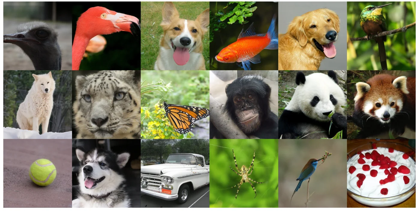 Selected samples from the best ImageNet 512×512 model (FID 3.85, guided base model plus upsampler). Figure from the paper.
Method
Architecture ablations
The starting point is the UNet from DDPM / Improved DDPM, with learned reverse-process variances and the hybrid objective \(L_{\text{simple}} + \lambda L_{\text{vlb}}\). On ImageNet 128×128 (batch 256, 250 sampling steps), the authors ablate one change at a time. Relative to the baseline (160 channels, 2 residual blocks, 1 head, attention at 16×16; FID 15.33 at 700K and 13.21 at 1200K iterations):
- depth 4 at 128 channels: −0.21 / −0.48, but slower in wall-clock time, so it is dropped
- 4 attention heads: −0.54 / −0.82
- attention at 32, 16 and 8 resolution: −0.72 / −0.66
- BigGAN residual blocks for up/downsampling: −1.20 / −1.21
- rescaling residual connections by \(1/\sqrt{2}\): +0.16 / +0.25 (worse)
- heads, multi-resolution attention and BigGAN up/down combined: −3.14 / −3.00
More heads or fewer channels per head both help, and 64 channels per head is chosen as the best in wall-clock time. Timestep and class embeddings enter each residual block through adaptive group normalization, \(\mathrm{AdaGN}(h, y) = y_s\, \mathrm{GroupNorm}(h) + y_b\), which gives FID 13.06 versus 15.08 for the addition-plus-GroupNorm layer of DDPM. The final ADM uses variable width, 2 residual blocks per resolution, 64 channels per head, attention at 32/16/8, BigGAN up/downsampling, and AdaGN.
Classifier guidance
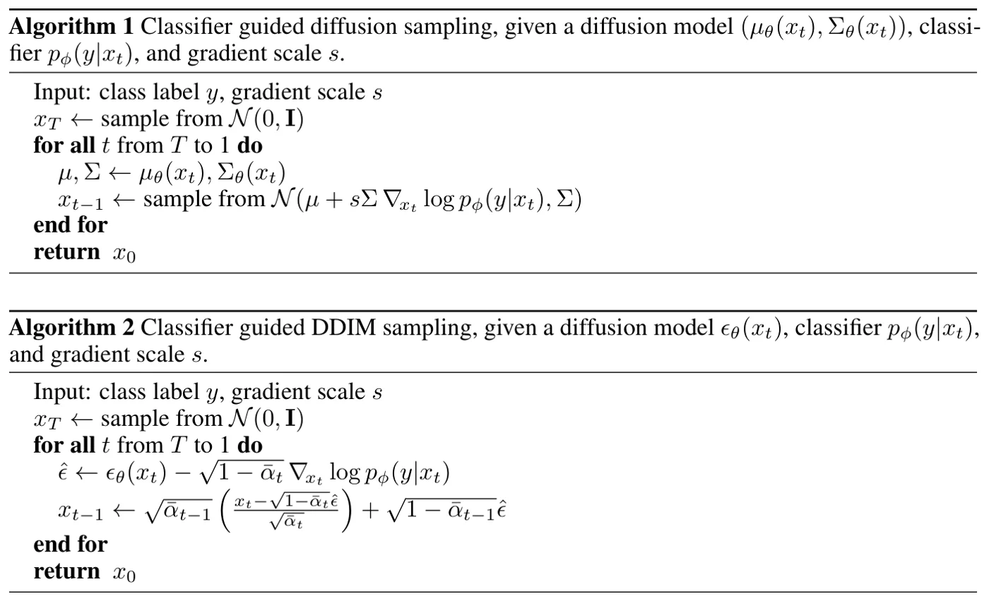 Algorithm 1: classifier-guided ancestral sampling, which shifts the mean of each Gaussian step by \(s\Sigma\nabla \log p_\phi(y \mid x_t)\). Algorithm 2: the DDIM version, which shifts the predicted noise instead. Figure from the paper.
To sample conditionally on a label \(y\), each reverse step should follow \(p_{\theta,\phi}(x_t \mid x_{t+1}, y) = Z\, p_\theta(x_t \mid x_{t+1})\, p_\phi(y \mid x_t)\). The diffusion step is a Gaussian \(\mathcal N(\mu, \Sigma)\). If \(\log p_\phi(y \mid x_t)\) has low curvature relative to \(\Sigma^{-1}\), a first-order Taylor expansion around \(x_t = \mu\) with \(g = \nabla_{x_t} \log p_\phi(y \mid x_t)\rvert_{x_t=\mu}\) gives
\[\log\big(p_\theta(x_t \mid x_{t+1})\, p_\phi(y \mid x_t)\big) \approx \log p(z) + C, \qquad z \sim \mathcal N(\mu + \Sigma g,\ \Sigma)\]So conditioning just shifts the mean of each step by \(\Sigma g\). For deterministic DDIM sampling, the paper uses the score view instead. Since \(\nabla_{x_t} \log p_\theta(x_t) = -\epsilon_\theta(x_t)/\sqrt{1-\bar\alpha_t}\), the noise prediction for the joint \(p(x_t)\,p(y \mid x_t)\) is
\[\hat\epsilon(x_t) = \epsilon_\theta(x_t) - \sqrt{1-\bar\alpha_t}\, \nabla_{x_t} \log p_\phi(y \mid x_t)\]and the usual DDIM update is run with \(\hat\epsilon\).
The classifier is the downsampling half of the UNet with an attention pool at 8×8. It is trained on noisy images from the same noising distribution as the diffusion model, with random crops against overfitting.
Gradient scale. With scale 1, an unconditional model guided toward “Pembroke Welsh corgi” produced samples to which the classifier assigned about 50% probability but which did not look like corgis. Multiplying the gradient by \(s > 1\) fixes this. Since \(s \nabla_x \log p(y \mid x) = \nabla_x \log \tfrac{1}{Z} p(y \mid x)^s\), guidance with scale \(s\) samples from a model conditioned on a sharpened classifier \(\propto p(y \mid x)^s\), which concentrates on the classifier’s modes: higher fidelity, lower diversity.
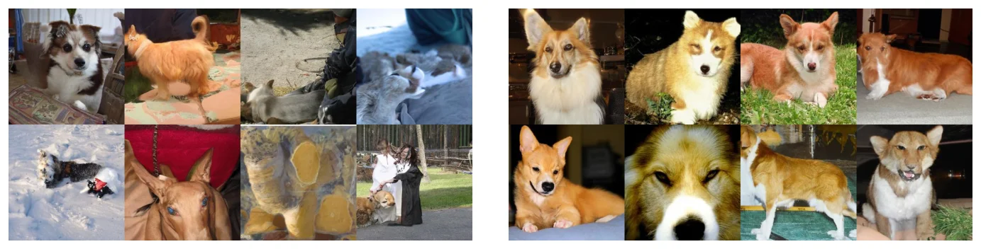 Unconditional ImageNet model guided to “Pembroke Welsh corgi”. Scale 1.0 (left, FID 33.0) gives mostly off-class images; scale 10.0 (right, FID 12.0) gives clearly class-consistent ones. Figure from the paper.
Guidance also works on top of a class-conditional model, and that combination gives the best results.
Main Experiments
Effect of classifier guidance on ImageNet 256×256 (both models trained for 2M iterations, batch 256):
| Conditional | Guidance scale | FID ↓ | sFID ↓ | IS ↑ | Precision ↑ | Recall ↑ |
|---|---|---|---|---|---|---|
| no | none | 26.21 | 6.35 | 39.70 | 0.61 | 0.63 |
| no | 1.0 | 33.03 | 6.99 | 32.92 | 0.56 | 0.65 |
| no | 10.0 | 12.00 | 10.40 | 95.41 | 0.76 | 0.44 |
| yes | none | 10.94 | 6.02 | 100.98 | 0.69 | 0.63 |
| yes | 1.0 | 4.59 | 5.25 | 186.70 | 0.82 | 0.52 |
| yes | 10.0 | 9.11 | 10.93 | 283.92 | 0.88 | 0.32 |
Comparison with the state of the art on class-conditional ImageNet (ADM-G = ADM with classifier guidance; 250 sampling steps unless noted):
| Resolution | Model | FID ↓ | sFID ↓ | Precision ↑ | Recall ↑ |
|---|---|---|---|---|---|
| 128×128 | BigGAN-deep | 6.02 | 7.18 | 0.86 | 0.35 |
| ADM | 5.91 | 5.09 | 0.70 | 0.65 | |
| ADM-G (25 steps) | 5.98 | 7.04 | 0.78 | 0.51 | |
| ADM-G | 2.97 | 5.09 | 0.78 | 0.59 | |
| 256×256 | BigGAN-deep | 6.95 | 7.36 | 0.87 | 0.28 |
| ADM | 10.94 | 6.02 | 0.69 | 0.63 | |
| ADM-G (25 steps) | 5.44 | 5.32 | 0.81 | 0.49 | |
| ADM-G | 4.59 | 5.25 | 0.82 | 0.52 | |
| 512×512 | BigGAN-deep | 8.43 | 8.13 | 0.88 | 0.29 |
| ADM | 23.24 | 10.19 | 0.73 | 0.60 | |
| ADM-G (25 steps) | 8.41 | 9.67 | 0.83 | 0.47 | |
| ADM-G | 7.72 | 6.57 | 0.87 | 0.42 |
- Guidance is what moves ImageNet past BigGAN-deep: at 256×256 it takes the conditional model from FID 10.94 to 4.59, and recall stays well above BigGAN-deep’s (0.52 vs. 0.28). With only 25 DDIM steps, ADM-G already matches or beats BigGAN-deep FID at every resolution.
- The architecture alone is enough for unconditional LSUN and ImageNet 64×64: ADM (with dropout) gets FID 1.90 on LSUN Bedrooms (StyleGAN 2.35), 2.57 on Horses (StyleGAN2 3.84), 5.57 on Cats (StyleGAN2 7.25), and 2.07 on ImageNet 64×64 (BigGAN-deep 4.06).
- Guidance and upsampling are complementary. Guiding the low-resolution base model and then applying the ADM-U upsampler gives FID 3.94 at 256×256 (ADM-U alone 7.49) and 3.85 at 512×512 (ADM-U alone 9.96).
The gradient scale behaves like a clean fidelity-diversity knob. On a class-conditional ImageNet 128×128 model, raising the scale raises precision and IS and lowers recall monotonically, while FID and sFID are best at a small scale and then rise.
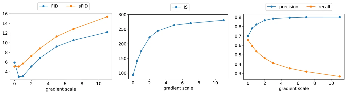 FID/sFID, IS, and precision/recall as the gradient scale grows from 0 to about 11, for a class-conditional ImageNet 128×128 model. Figure from the paper.
Against BigGAN-deep’s truncation trick, guidance gives a strictly better FID-IS curve. On precision-recall it is better only up to a precision of about 0.9; beyond that BigGAN-deep can reach higher precision, while guidance cannot.
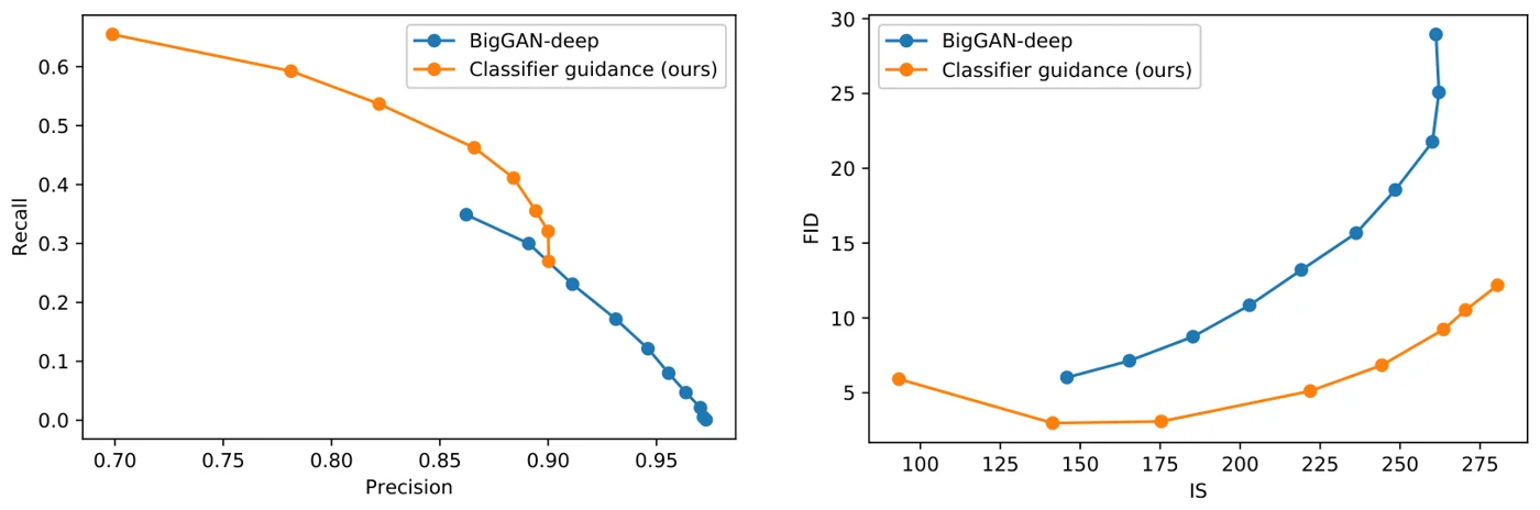 ImageNet 128×128. Left: precision vs. recall. Right: FID vs. IS. BigGAN-deep is swept over truncation 0.1 to 1.0, classifier guidance over the gradient scale. Figure from the paper.
Random samples show the coverage difference qualitatively: at similar perceptual quality, the guided diffusion model shows more modes than BigGAN-deep, such as close-up ostrich heads, single flamingos, and a tench without a person holding it.
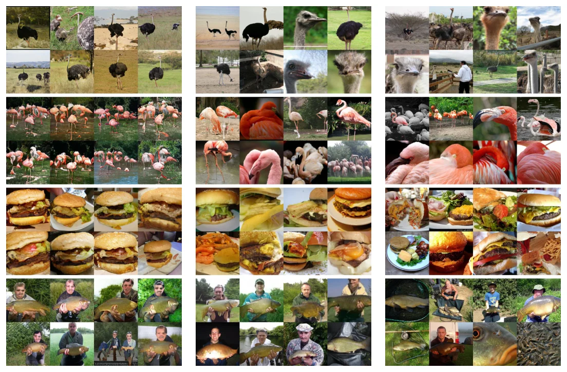 Random samples for ostrich, flamingo, cheeseburger, and tench. Left: BigGAN-deep, truncation 1.0 (FID 6.95). Middle: ADM-G (FID 4.59). Right: training images. Figure from the paper.
Limitations
- Sampling is slow. The headline numbers use 250 denoising steps (1000 for LSUN), each a full network pass, plus a classifier forward and backward pass when guiding. The paper names sampling speed as the main remaining gap to GANs.
- Labels are required. Classifier guidance needs a labeled dataset, and the paper offers no way to trade diversity for fidelity on unlabeled data.
- A second model must be trained. The classifier has to be trained on noisy images over all timesteps, so an off-the-shelf classifier cannot be plugged in, and guidance is limited to the label set that classifier knows.
- Fidelity costs coverage. Guidance improves FID mainly by raising precision. At 512×512, recall drops from 0.60 (ADM) to 0.42 (ADM-G), and at high scales it falls further while FID gets worse again.
- The Taylor-expansion argument is approximate. It assumes the classifier’s log-probability has low curvature relative to \(\Sigma^{-1}\), which holds in the limit of many small steps. With large scales, the method is a heuristic sharpening \(p(y \mid x)^s\) rather than exact conditional sampling.