Abstract
2021년 당시 대부분의 image generation benchmark에서 state of the art는 GAN이었고, diffusion model을 포함한 likelihood-based model은 data distribution을 더 잘 덮지만 sample fidelity가 낮았다. Diffusion model은 CIFAR-10에서는 이미 앞서 있었지만, ImageNet 같은 어려운 dataset에서는 여전히 BigGAN-deep에 뒤처졌다. 저자들은 그 차이를 두 가지로 설명한다. GAN architecture는 훨씬 더 많이 튜닝되어 왔고, GAN에는 diversity를 fidelity와 맞바꾸는 손잡이(truncation trick)가 있지만 diffusion model에는 없었다.
논문은 둘 다 해결한다. 일련의 ablation으로 개선된 UNet인 ADM(ablated diffusion model)을 얻는다. 이어서 classifier guidance가 noisy image로 학습한 classifier의 gradient를 각 sampling step에 더한다. 그 gradient에 곱하는 scale 하나로 diversity와 fidelity를 맞바꾼다. 결과는 ImageNet 128×128에서 FID 2.97, 256×256에서 4.59, 512×512에서 7.72로 모두 BigGAN-deep보다 좋으며, guidance를 upsampling stack과 결합하면 256과 512에서 각각 3.94와 3.85이다.
Motivation
논문은 GAN의 장단점을 중심으로 motivation을 구성한다. GAN은 FID, Inception Score, Precision으로 측정한 sample quality가 높지만, 이 metric들은 diversity를 충분히 반영하지 못하며 GAN은 likelihood-based model보다 distribution을 덜 덮는다는 것이 알려져 있다. 또한 학습이 어렵고, hyperparameter와 regularizer를 신중히 고르지 않으면 collapse한다. Diffusion model은 distribution coverage, 고정된(stationary) training objective, 쉬운 scaling을 제공하며, 같은 저자들의 이전 연구는 compute를 늘리면 꾸준히 좋아진다는 것을 보였다. 그러나 upsampling stack을 써도 ImageNet 256×256 FID는 BigGAN-deep에 미치지 못했다.
저자들의 가설은 이 차이가 근본적인 것이 아니라는 것이다. 첫째, diffusion UNet은 GAN backbone에 비해 architecture 탐색을 거의 거치지 않았다. 둘째, GAN(그리고 low-temperature sampling이나 rejection sampling을 쓰는 다른 likelihood model)은 diversity를 포기하고 fidelity를 얻을 수 있지만, diffusion model에는 그런 손잡이가 없었다. 두 격차를 모두 메우면 GAN을 앞지르기에 충분해야 한다. Teaser는 최종 모델이 512×512에서 생성하는 sample을 보여준다.
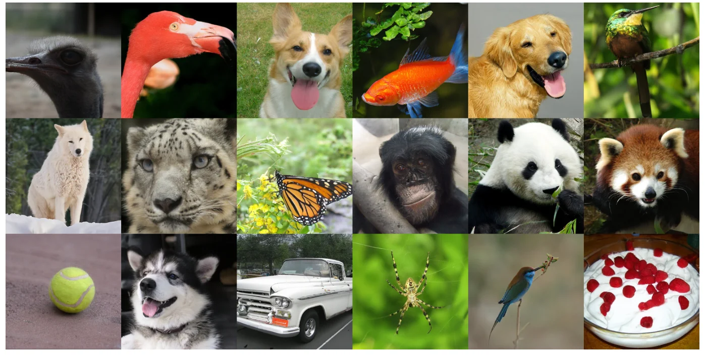 최고 성능 ImageNet 512×512 모델(FID 3.85, guidance를 적용한 base model과 upsampler)에서 고른 sample. 논문 Figure.
Method
Architecture ablations
출발점은 DDPM / Improved DDPM의 UNet으로, 학습된 reverse-process variance와 hybrid objective \(L_{\text{simple}} + \lambda L_{\text{vlb}}\)를 사용한다. ImageNet 128×128(batch 256, sampling step 250)에서 저자들은 변경을 하나씩 ablation한다. Baseline(channel 160, residual block 2개, head 1개, 16×16에서 attention; 700K iteration에서 FID 15.33, 1200K에서 13.21) 대비:
- channel 128에서 depth 4: −0.21 / −0.48. 그러나 wall-clock time 기준으로 느려 제외한다
- attention head 4개: −0.54 / −0.82
- 32, 16, 8 resolution에서 attention: −0.72 / −0.66
- up/downsampling에 BigGAN residual block 사용: −1.20 / −1.21
- residual connection을 \(1/\sqrt{2}\)로 rescale: +0.16 / +0.25(악화)
- head, multi-resolution attention, BigGAN up/down 결합: −3.14 / −3.00
Head를 늘리거나 head당 channel을 줄이는 것 모두 도움이 되며, wall-clock time 기준으로 가장 좋은 head당 64 channel을 선택한다. Timestep과 class embedding은 adaptive group normalization \(\mathrm{AdaGN}(h, y) = y_s\, \mathrm{GroupNorm}(h) + y_b\)를 통해 각 residual block에 들어가며, DDPM의 addition + GroupNorm layer(FID 15.08)보다 좋은 FID 13.06을 얻는다. 최종 ADM은 가변 width, resolution당 residual block 2개, head당 64 channel, 32/16/8에서의 attention, BigGAN up/downsampling, AdaGN을 사용한다.
Classifier guidance
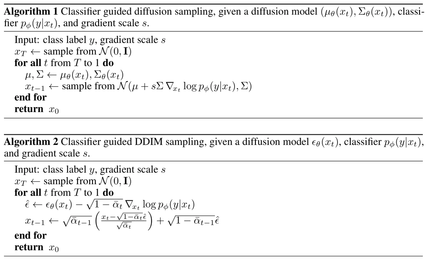 Algorithm 1: classifier-guided ancestral sampling으로, 각 Gaussian step의 평균을 \(s\Sigma\nabla \log p_\phi(y \mid x_t)\)만큼 이동시킨다. Algorithm 2: DDIM 버전으로, 대신 예측된 noise를 이동시킨다. 논문 Figure.
Label \(y\)로 조건부 sampling을 하려면 각 reverse step이 \(p_{\theta,\phi}(x_t \mid x_{t+1}, y) = Z\, p_\theta(x_t \mid x_{t+1})\, p_\phi(y \mid x_t)\)를 따라야 한다. Diffusion step은 Gaussian \(\mathcal N(\mu, \Sigma)\)이다. \(\log p_\phi(y \mid x_t)\)의 curvature가 \(\Sigma^{-1}\)에 비해 작다면, \(g = \nabla_{x_t} \log p_\phi(y \mid x_t)\rvert_{x_t=\mu}\)로 \(x_t = \mu\) 주변에서 1차 Taylor 전개를 하여 다음을 얻는다.
\[\log\big(p_\theta(x_t \mid x_{t+1})\, p_\phi(y \mid x_t)\big) \approx \log p(z) + C, \qquad z \sim \mathcal N(\mu + \Sigma g,\ \Sigma)\]즉 conditioning은 각 step의 평균을 \(\Sigma g\)만큼 옮기는 것에 불과하다. Deterministic DDIM sampling에 대해서는 score 관점을 사용한다. \(\nabla_{x_t} \log p_\theta(x_t) = -\epsilon_\theta(x_t)/\sqrt{1-\bar\alpha_t}\)이므로, joint \(p(x_t)\,p(y \mid x_t)\)에 대한 noise prediction은 다음과 같다.
\[\hat\epsilon(x_t) = \epsilon_\theta(x_t) - \sqrt{1-\bar\alpha_t}\, \nabla_{x_t} \log p_\phi(y \mid x_t)\]그리고 \(\hat\epsilon\)로 일반 DDIM update를 실행한다.
Classifier는 UNet의 downsampling 절반에 8×8에서 attention pool을 붙인 것이다. Diffusion model과 같은 noising distribution의 noisy image로 학습하며, overfitting을 막기 위해 random crop을 사용한다.
Gradient scale. Scale 1로 unconditional model을 “Pembroke Welsh corgi” 쪽으로 guide하면, classifier는 약 50%의 확률을 주지만 눈으로 보면 corgi가 아닌 sample이 나왔다. Gradient에 \(s > 1\)을 곱하면 이 문제가 해결된다. \(s \nabla_x \log p(y \mid x) = \nabla_x \log \tfrac{1}{Z} p(y \mid x)^s\)이므로, scale \(s\)의 guidance는 날카로워진 classifier \(\propto p(y \mid x)^s\)로 조건부화된 모델에서 sampling하는 것이며, 이는 classifier의 mode에 집중한다. 즉 fidelity는 높아지고 diversity는 낮아진다.
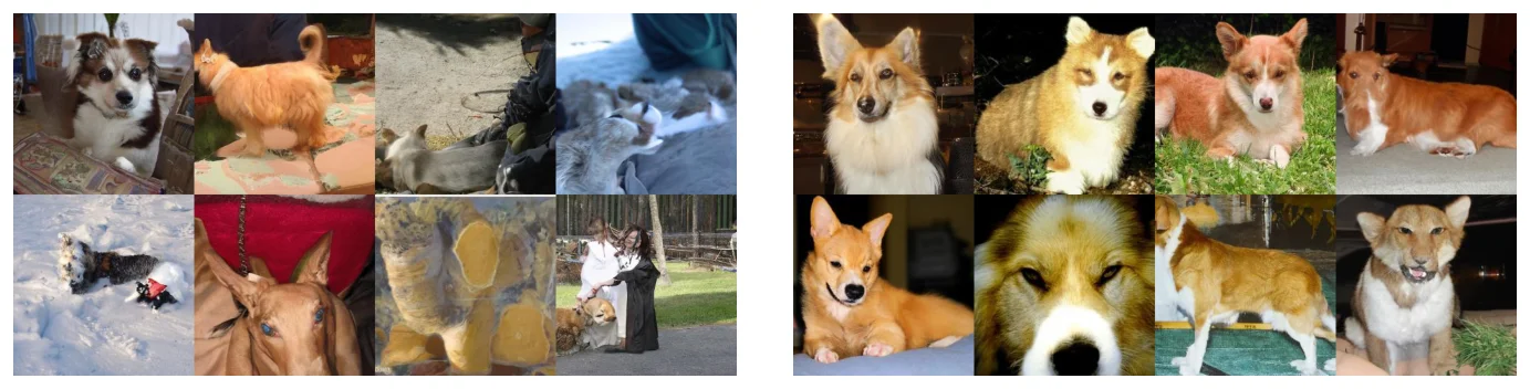 “Pembroke Welsh corgi”로 guide한 unconditional ImageNet 모델. Scale 1.0(왼쪽, FID 33.0)은 대부분 class와 맞지 않는 image를, scale 10.0(오른쪽, FID 12.0)은 class에 분명히 부합하는 image를 낸다. 논문 Figure.
Guidance는 class-conditional model 위에서도 동작하며, 그 조합이 가장 좋은 결과를 낸다.
Main Experiments
ImageNet 256×256에서 classifier guidance의 효과(두 모델 모두 2M iteration, batch 256으로 학습):
| Conditional | Guidance scale | FID ↓ | sFID ↓ | IS ↑ | Precision ↑ | Recall ↑ |
|---|---|---|---|---|---|---|
| no | none | 26.21 | 6.35 | 39.70 | 0.61 | 0.63 |
| no | 1.0 | 33.03 | 6.99 | 32.92 | 0.56 | 0.65 |
| no | 10.0 | 12.00 | 10.40 | 95.41 | 0.76 | 0.44 |
| yes | none | 10.94 | 6.02 | 100.98 | 0.69 | 0.63 |
| yes | 1.0 | 4.59 | 5.25 | 186.70 | 0.82 | 0.52 |
| yes | 10.0 | 9.11 | 10.93 | 283.92 | 0.88 | 0.32 |
Class-conditional ImageNet에서 state of the art와의 비교(ADM-G = classifier guidance를 쓴 ADM; 별도 표기가 없으면 sampling step 250):
| Resolution | Model | FID ↓ | sFID ↓ | Precision ↑ | Recall ↑ |
|---|---|---|---|---|---|
| 128×128 | BigGAN-deep | 6.02 | 7.18 | 0.86 | 0.35 |
| ADM | 5.91 | 5.09 | 0.70 | 0.65 | |
| ADM-G (25 steps) | 5.98 | 7.04 | 0.78 | 0.51 | |
| ADM-G | 2.97 | 5.09 | 0.78 | 0.59 | |
| 256×256 | BigGAN-deep | 6.95 | 7.36 | 0.87 | 0.28 |
| ADM | 10.94 | 6.02 | 0.69 | 0.63 | |
| ADM-G (25 steps) | 5.44 | 5.32 | 0.81 | 0.49 | |
| ADM-G | 4.59 | 5.25 | 0.82 | 0.52 | |
| 512×512 | BigGAN-deep | 8.43 | 8.13 | 0.88 | 0.29 |
| ADM | 23.24 | 10.19 | 0.73 | 0.60 | |
| ADM-G (25 steps) | 8.41 | 9.67 | 0.83 | 0.47 | |
| ADM-G | 7.72 | 6.57 | 0.87 | 0.42 |
- ImageNet에서 BigGAN-deep을 넘어서게 하는 것은 guidance이다. 256×256에서 conditional model의 FID를 10.94에서 4.59로 낮추며, recall은 BigGAN-deep보다 훨씬 높게 유지된다(0.52 vs. 0.28). DDIM step 25개만으로도 ADM-G는 모든 resolution에서 BigGAN-deep의 FID와 같거나 더 낫다.
- Unconditional LSUN과 ImageNet 64×64에서는 architecture만으로 충분하다. ADM(dropout 적용)은 LSUN Bedrooms에서 FID 1.90(StyleGAN 2.35), Horses에서 2.57(StyleGAN2 3.84), Cats에서 5.57(StyleGAN2 7.25), ImageNet 64×64에서 2.07(BigGAN-deep 4.06)을 얻는다.
- Guidance와 upsampling은 상호 보완적이다. 저해상도 base model을 guide한 뒤 ADM-U upsampler를 적용하면 256×256에서 FID 3.94(ADM-U 단독 7.49), 512×512에서 3.85(ADM-U 단독 9.96)를 얻는다.
Gradient scale은 깔끔한 fidelity-diversity 손잡이처럼 동작한다. Class-conditional ImageNet 128×128 모델에서 scale을 키우면 precision과 IS는 오르고 recall은 단조롭게 떨어지며, FID와 sFID는 작은 scale에서 최적이 된 뒤 다시 오른다.
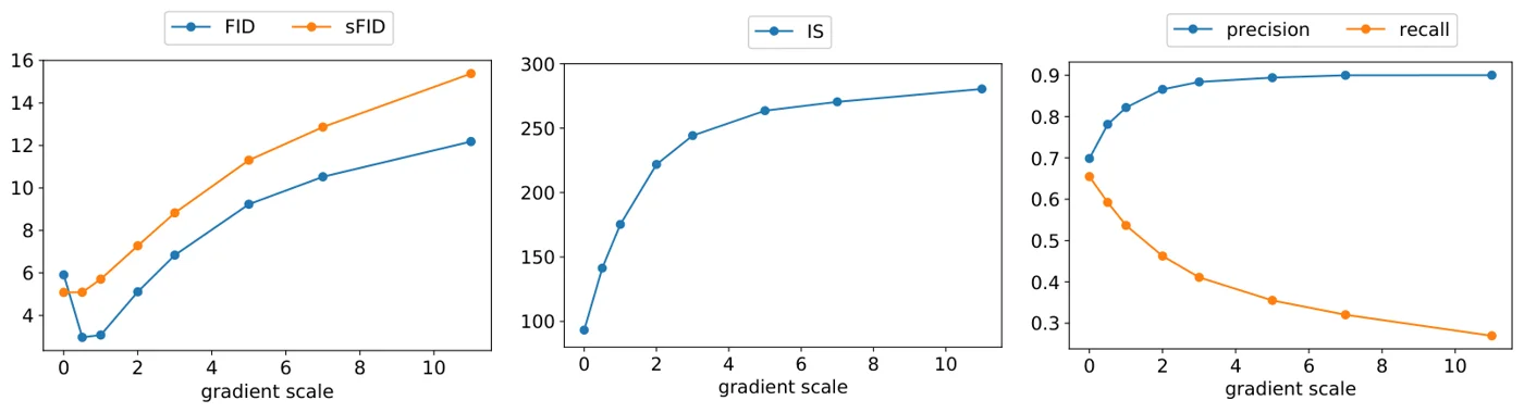 Class-conditional ImageNet 128×128 모델에서 gradient scale을 0에서 약 11까지 키울 때의 FID/sFID, IS, precision/recall. 논문 Figure.
BigGAN-deep의 truncation trick과 비교하면, guidance는 FID-IS 곡선에서 엄격하게 더 낫다. Precision-recall에서는 precision 약 0.9까지만 더 나으며, 그 이상에서는 BigGAN-deep이 더 높은 precision에 도달할 수 있지만 guidance는 그렇지 못하다.
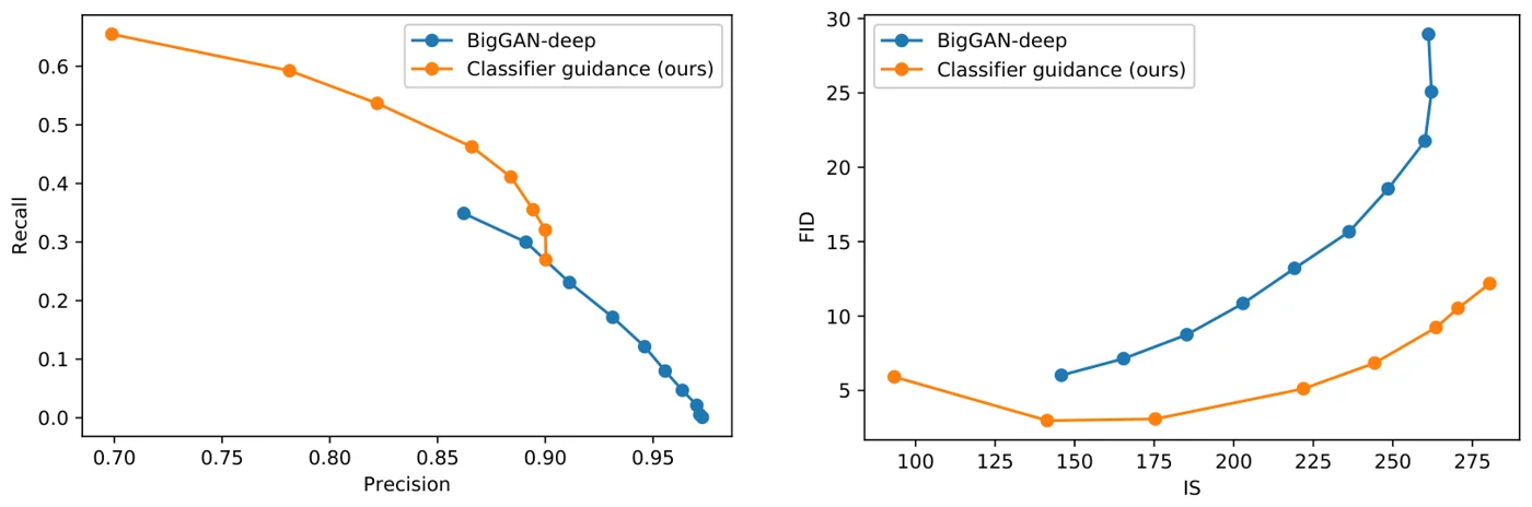 ImageNet 128×128. 왼쪽: precision vs. recall. 오른쪽: FID vs. IS. BigGAN-deep은 truncation 0.1~1.0, classifier guidance는 gradient scale을 바꿔 가며 측정한다. 논문 Figure.
Random sample은 coverage 차이를 정성적으로 보여준다. 비슷한 perceptual quality에서 guided diffusion model은 BigGAN-deep보다 더 많은 mode를 보인다. 예를 들어 타조 머리 close-up, 홀로 있는 홍학, 사람이 들고 있지 않은 tench 등이다.
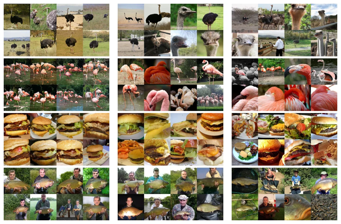 타조, 홍학, cheeseburger, tench의 random sample. 왼쪽: BigGAN-deep, truncation 1.0(FID 6.95). 가운데: ADM-G(FID 4.59). 오른쪽: training image. 논문 Figure.
Limitations
- Sampling이 느리다. 주요 수치는 denoising step 250개(LSUN은 1000개)를 사용하며, 각 step이 network 전체 pass이고 guidance 시에는 classifier의 forward와 backward pass가 추가된다. 논문은 sampling 속도를 GAN과의 주요 남은 격차로 꼽는다.
- Label이 필요하다. Classifier guidance는 labeled dataset이 필요하며, 논문은 unlabeled data에서 diversity와 fidelity를 맞바꾸는 방법을 제시하지 않는다.
- 두 번째 모델을 학습해야 한다. Classifier는 모든 timestep의 noisy image로 학습해야 하므로 기성 classifier를 그대로 꽂아 쓸 수 없고, guidance는 그 classifier가 아는 label 집합으로 제한된다.
- Fidelity는 coverage를 대가로 한다. Guidance는 주로 precision을 높여 FID를 개선한다. 512×512에서 recall은 0.60(ADM)에서 0.42(ADM-G)로 떨어지며, 큰 scale에서는 더 떨어지고 FID도 다시 나빠진다.
- Taylor 전개 논증은 근사이다. Classifier의 log-probability curvature가 \(\Sigma^{-1}\)에 비해 작다고 가정하는데, 이는 작은 step이 많은 극한에서 성립한다. 큰 scale에서는 정확한 조건부 sampling이라기보다 \(p(y \mid x)^s\)로 날카롭게 만드는 heuristic이다.