Abstract
Test-time adaptation (TTA) for 3D point clouds usually updates the model with backpropagation. Pseudo-label methods can feed noisy labels back into the model, so errors pile up over the test stream and source knowledge is forgotten. Self-supervised methods such as MATE work better but are slow, which is a problem when adaptation must happen on the fly.
BFTT3D never updates the source model. It adds a second branch built from parameter-free parts: a non-parametric point cloud encoder, a small memory of source prototypes, and a closed-form subspace alignment. This branch produces a target-specific logit. It is mixed with the frozen source model’s logit using a weight computed from the two prediction entropies.
Motivation
The paper’s motivation is a trade-off between the two main families of 3D TTA. Pseudo-label methods (often teacher-student schemes) are fast, but every update is supervised by labels the model produced itself. Wrong labels are fed back by backpropagation, errors build up across the stream, and source knowledge is overwritten. Self-supervised methods such as MATE avoid noisy labels and work better, but they need an auxiliary task and gradient updates at test time, which the authors consider too slow for something like a LiDAR detector that must adapt as the weather changes. The ScanObjectNN-C results later in the paper show how badly the first family can fail on small real-scanned data: SHOT raises CurveNet’s error from 64.77 to 85.35.
The authors’ answer is to keep the source model completely frozen, so nothing can be forgotten, and to put all target-specific information into a branch that has no trainable parameters at all. The figure below contrasts the two pipelines: the baseline sends gradients from pseudo-labels back into the source model, while BFTT3D runs the frozen model next to a backpropagation-free module and only fuses their outputs.
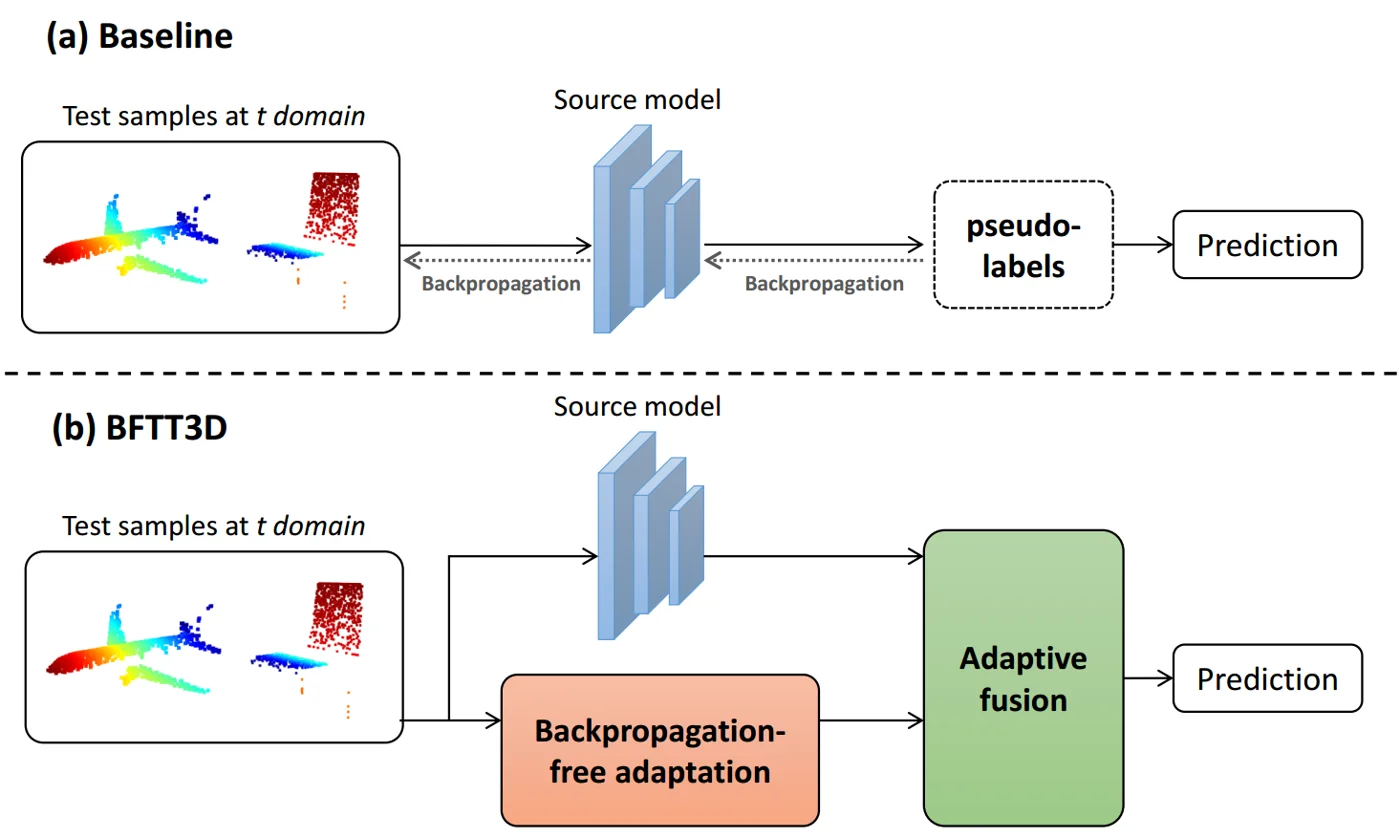 (a) Typical 3D TTA: the source model produces pseudo-labels and is trained on them by backpropagation. (b) BFTT3D: the source model stays frozen, a backpropagation-free adaptation module produces a second prediction, and adaptive fusion combines the two. Figure from the paper.
Method
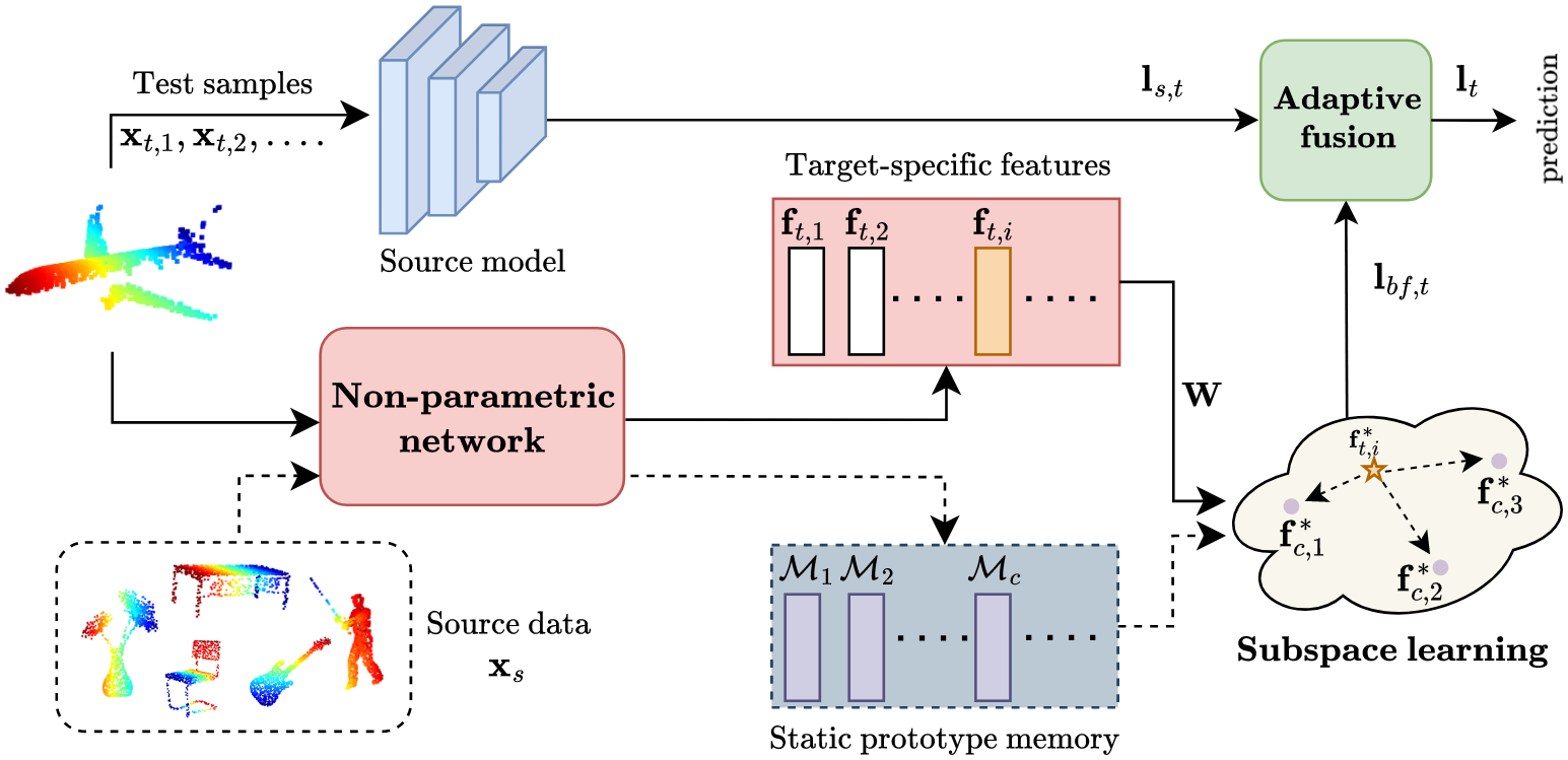 Two streams: the frozen source model gives \(\mathbf{l}_{s,t}\), and a non-parametric network plus subspace matching against a static prototype memory gives \(\mathbf{l}_{bf,t}\). Adaptive fusion combines them into \(\mathbf{l}_t\). Figure from the paper.
The source model \(h_{\theta_s}\) is a standard pre-trained classifier (PointNet, DGCNN or CurveNet). It is frozen and gives the source-specific logit \(\mathbf{l}_{s,t}\). Everything else in the figure exists to produce a second logit, \(\mathbf{l}_{bf,t}\), without any trainable weights.
Non-parametric network
The lower branch uses the non-parametric encoder from Point-NN. It has no learned weights. It is built only from farthest point sampling, \(k\)-NN grouping, pooling, and trigonometric position embeddings. Each coordinate is encoded with sines and cosines, neighbour features are concatenated to each center and reweighted by a relative-position encoding, and max plus average pooling condense each group. This is repeated four times, and a global pooling gives a feature \(\mathbf{f}_{t,i} \in \mathbb{R}^d\) for each test sample. Because nothing is trained, the authors argue this encoder is less biased toward the source domain.
Static prototype memory
Before test time, the same encoder is run on the source data. For each class \(c\), a herding algorithm keeps the features closest to the class mean, giving a fixed memory \(\mathcal{M}_c\). The paper keeps 25% of the source features. This memory is built once and never changes.
Subspace learning
Matching target features directly against source prototypes would suffer from the domain gap. So both are first projected into a shared subspace, \(\mathbf{f}^* = \psi(\mathbf{f})\), chosen to minimize the Maximum Mean Discrepancy (MMD) between prototypes and test features:
\[\operatorname{Dist}(\mathcal{Q}_s, \mathcal{Q}_t) = \left\| \frac{1}{n_s}\sum_{i=1}^{n_s} \mathbf{f}_i^* - \frac{1}{n_t}\sum_{i=1}^{n_t} \mathbf{f}_{t,i}^* \right\|_{\mathcal{H}}^2\]The projection is found with Transfer Component Analysis (TCA). With a kernel matrix \(\mathbf{K}\) over all \(n_s + n_t\) prototype and test features, a scaling matrix \(\mathbf{L}\) and a centering matrix \(\mathbf{H}\), TCA solves
\[\min_{\mathbf{W}} \operatorname{tr}(\mathbf{W}^T \mathbf{K}\mathbf{L}\mathbf{K}\mathbf{W}) + \mu \operatorname{tr}(\mathbf{W}^T\mathbf{W}) \quad \text{s.t. } \mathbf{W}^T\mathbf{K}\mathbf{H}\mathbf{K}\mathbf{W} = \mathbf{I}\]The solution is closed form: the \(m\) leading eigenvectors of \((\mathbf{KLK} + \mu\mathbf{I})^{-1}\mathbf{KHK}\). The projected features are the columns of \(\mathbf{W}^T\mathbf{K}\), with \(m = 150\) in the paper. No gradient step is involved.
In the subspace, test features are compared with the prototypes by cosine similarity, \(\mathcal{J} = \tilde{\mathbf{F}}_t \cdot \tilde{\mathcal{M}}^T\), and turned into class scores with the prototype labels \(\mathbf{L}_m\):
\[\mathbf{l}_{bf,t} = \varphi(\mathcal{J}\mathbf{L}_m), \qquad \varphi(x) = \exp(-\gamma(1 - x))\]Adaptive fusion
The two logits are mixed with a weight \(p\):
\[\mathbf{l}_t = p \cdot \mathbf{l}_{bf,t} + (1-p) \cdot \mathbf{l}_{s,t}, \qquad p = 1 - \frac{\text{E}(\mathbf{l}_{bf,t})}{\text{E}(\mathbf{l}_{s,t}) + \text{E}(\mathbf{l}_{bf,t})}\]where \(\text{E}(\cdot)\) is the softmax entropy. When the source model is uncertain (high entropy), \(p\) grows and the prototype branch gets more weight. When the target is close to the source, the source model dominates. In an ablation, this adaptive \(p\) stays close to the best fixed \(p\) found by exhaustive search, without needing validation data.
Main Experiments
Mean classification error (%, lower is better) over 15 corruptions at severity 5. Each backbone is trained on the clean set and used as the source model. LAME and DSS are reported only with PointNet. This is a subset of Tables 1 and 2; the paper also lists per-corruption errors.
ModelNet-40C (Table 1)
| Method | PointNet | DGCNN | CurveNet |
|---|---|---|---|
| Source-only | 35.88 | 34.65 | 28.47 |
| TENT | 34.62 | 30.99 | 22.60 |
| BN | 34.89 | 31.36 | 24.03 |
| SHOT | 34.25 | 30.17 | 19.79 |
| LAME | 83.16 | – | – |
| DSS | 35.23 | – | – |
| BFTT3D | 33.78 | 29.33 | 19.23 |
ScanObjectNN-C (Table 2)
| Method | PointNet | DGCNN | CurveNet |
|---|---|---|---|
| Source-only | 59.35 | 46.09 | 64.77 |
| TENT | 58.18 | 45.17 | 65.77 |
| BN | 57.87 | 45.11 | 64.26 |
| SHOT | 65.63 | 57.53 | 85.35 |
| LAME | 55.67 | – | – |
| DSS | 56.53 | – | – |
| BFTT3D | 54.46 | 43.91 | 57.80 |
BFTT3D has the lowest mean error in all six settings. On ModelNet-40C the margin over the best baseline is small (for example 19.23 vs. 19.79 for SHOT on CurveNet). On the smaller, real-scanned ScanObjectNN-C it is larger, because backpropagation baselines often fail to improve or even get worse there (SHOT rises to 85.35 on CurveNet). Gains concentrate on large shifts such as background, occlusion and LiDAR. The paper does not report runtime or memory numbers.
The full per-corruption tables show where the averages come from. On ModelNet-40C with PointNet, most columns move by less than one point, and the mean gain is carried by background (95.30 to 80.75), rotation (72.81 to 68.56) and LiDAR (59.00 to 55.88). Shear with DGCNN is one of the cells where BFTT3D is worse than the source model.
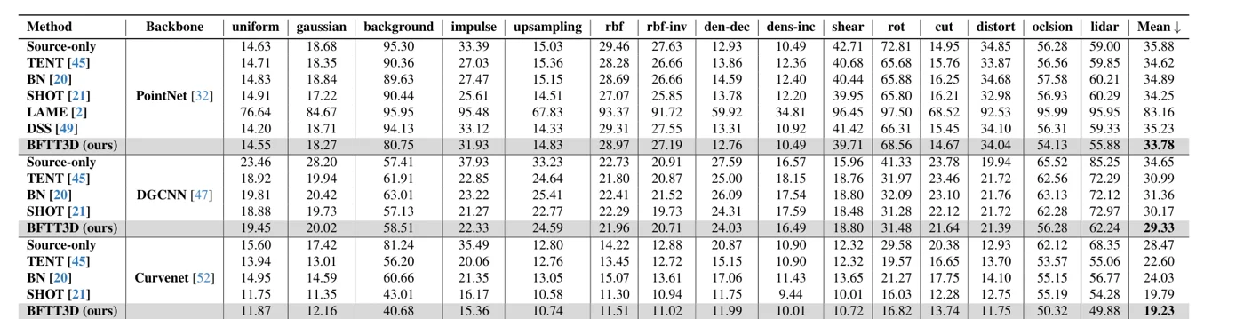 Table 1 of the paper: classification error (%) per corruption on ModelNet-40C for PointNet, DGCNN and CurveNet. BFTT3D rows are shaded; most gains are a few points, with the largest on background noise. Figure from the paper.
On ScanObjectNN-C the baselines are much less stable. SHOT is worse than the source model for all three backbones, while BFTT3D improves almost every column. With CurveNet the background error goes from 81.93 to 68.85 and density decrease from 35.46 to 30.29.
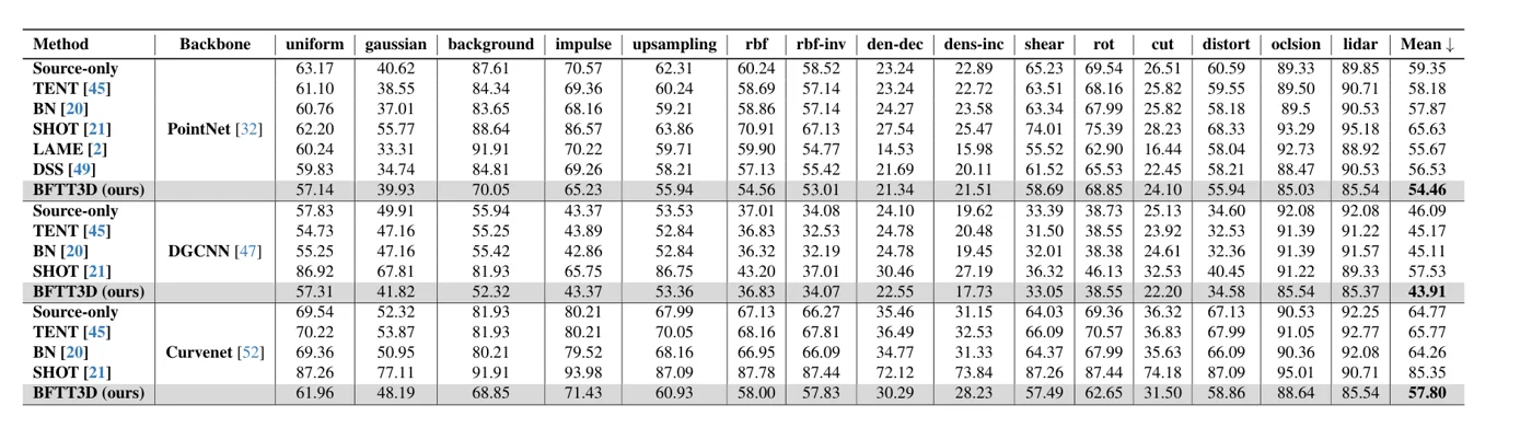 Table 2 of the paper: classification error (%) per corruption on ScanObjectNN-C. Note SHOT’s large increases (for example CurveNet impulse 93.98) next to BFTT3D’s steady gains. Figure from the paper.
The ablation on the fusion weight checks whether the entropy-based \(p\) is a reasonable substitute for tuning. For every corruption type, the error with the adaptive \(p\) stays a few points above the error with the best fixed \(p\) found by exhaustive search, and the two curves have the same shape.
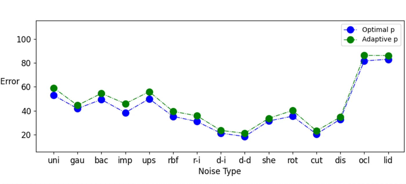 Error per corruption type with the optimal fixed \(p\) from exhaustive search (blue) and the entropy-based adaptive \(p\) (green), PointNet on ModelNet40-C. The adaptive ratio tracks the oracle closely without validation data. Figure from the paper.
Limitations
- Source data at test time. The prototype memory is built from source features (25% of them by default). This does not fit a strictly source-free setting.
- Per-batch TCA. The subspace is solved from a kernel matrix over all prototypes plus the current test features, followed by a matrix inverse and an eigen-decomposition. The cost grows with the memory size. The paper gives no timing. A later paper (Purge-Gate, ICCV 2025) measured 173.94 ms per batch and 7400 MiB of GPU memory for BFTT3D on a Point-MAE backbone.
- Needs a batch of test samples. The MMD/TCA step aligns a set of \(n_t\) test features with the prototypes. The test batch size used is not stated, and single-sample behaviour is not studied.
- Small gains on ModelNet-40C. With PointNet the mean error drops from 35.88 to 33.78. The method can also be worse than the source model on individual corruptions (shear on ModelNet-40C with DGCNN: 15.96 to 18.80).
- Two encoders at inference. Every test sample goes through both the source model and the non-parametric network.