Abstract
Point clouds from real sensors come with noise, occlusion, density changes and misalignment. A classifier trained on clean point clouds loses a lot of accuracy on them. Most test-time adaptation (TTA) methods update model parameters from the model’s own predictions, for example by entropy minimization. On point clouds this breaks down in realistic settings: with batch size 1, a label-sorted test stream, or class imbalance, TENT and SHOT collapse to about 4% accuracy. DDA, a 2D method, adapts the input with a diffusion model instead. Ported to 3D, it ignores point-cloud geometry and takes about 23.6 seconds per sample, because it runs a full generation process and backpropagates through the diffusion model.
CloudFixer also adapts the input, one sample at a time, but it does not regenerate the point cloud. It optimizes a small geometric transformation (a rotation plus per-point displacements) of the input. The target for this optimization is the one-step denoised estimate from a frozen source diffusion model. The diffusion model only runs forward passes. An optional online variant, CloudFixer-O, also updates the classifier so that its prediction on the original input agrees with its prediction on the adapted input.
Motivation
The authors first check how well standard model-update TTA transfers to point clouds. Figure 1 sweeps TENT’s batch size on ModelNet40-C with Point2Vec. With a randomly ordered stream, TENT needs a batch of about 8 just to match the unadapted model (about 62%) and only reaches CloudFixer’s level at batch size 64; at batch sizes 1 and 2 it collapses to a few percent. With a class-ordered stream it stays below about 13% at every batch size. The paper attributes this to the heavy reliance on the model’s own unstable predictions, which become biased when a batch is tiny or contains one class.
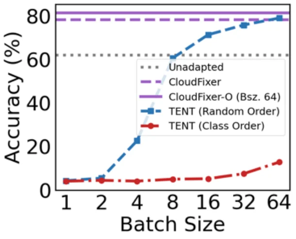 Accuracy of TENT on ModelNet40-C as the batch size grows, for a random-order and a class-order test stream, against the unadapted model and CloudFixer. TENT is useless at small batches and under class-ordered streams, while per-sample CloudFixer does not depend on either. Figure from the paper.
Input adaptation sidesteps this because it works on one sample and never trusts a pseudo-label. DDA showed this in 2D, but its recipe (add noise, then run the full reverse diffusion to regenerate the input) fits images, not point clouds. Many 3D corruptions are geometric, such as a rotated object or a few stray points, so regenerating every point is unnecessary and can erase shape detail, and the full reverse process with backpropagation through the diffusion model costs about 23.6 s per sample. The insight CloudFixer builds on is that a frozen diffusion model’s one-step estimate is enough to say which way the input should move, and that the move itself can be a small, structured transform (a rotation plus regularized per-point offsets) instead of a new sample.
Method
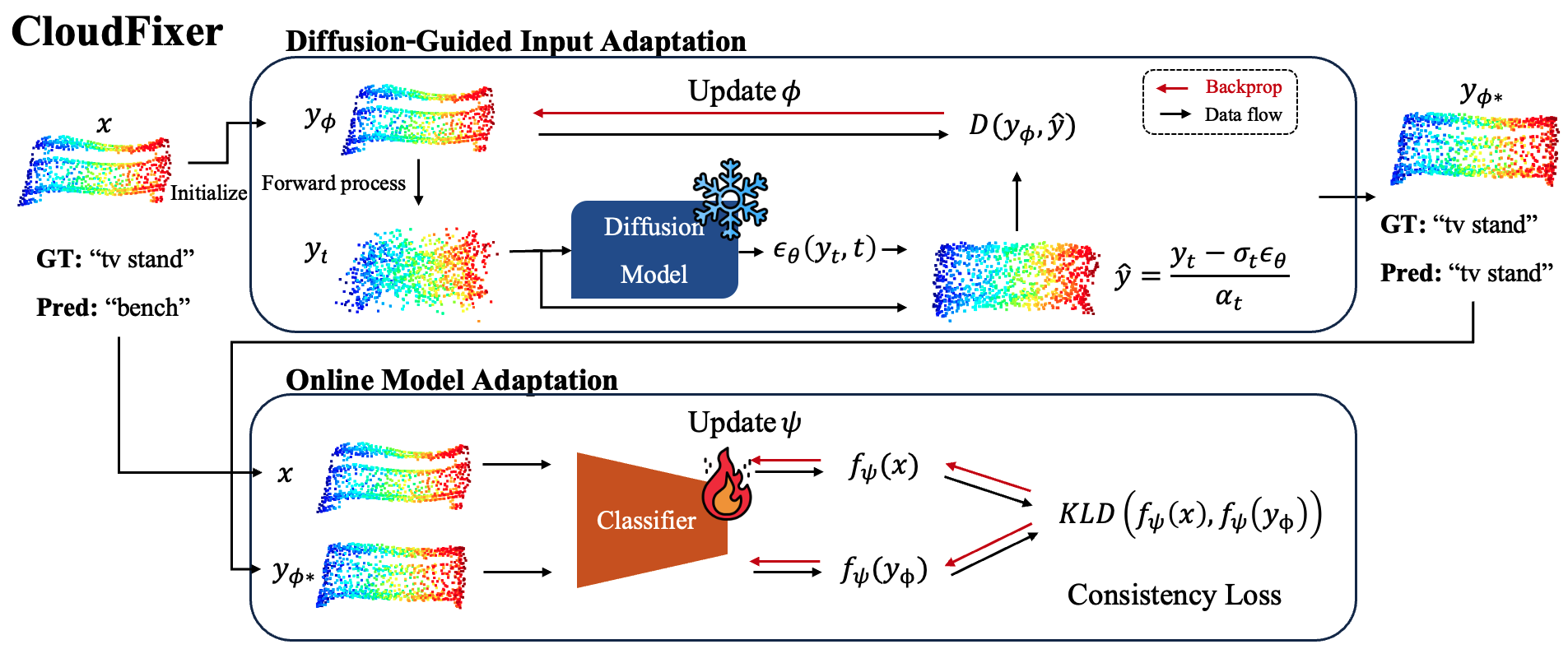 Top: diffusion-guided input adaptation optimizes the transformation parameters \(\phi\) so that \(y_\phi\) moves toward the diffusion model’s estimate \(\hat y\). Bottom: optional online model adaptation with a KL consistency loss between \(f_\psi(x)\) and \(f_\psi(y_{\phi^*})\). Figure from the paper.
Setup
A classifier \(f_\psi\) is trained on source point clouds \(x \in \mathbb{R}^{N \times 3}\). A diffusion model \(\epsilon_\theta\) is also trained on the source data, with \(x_t = \alpha_t x_0 + \sigma_t \epsilon\). From a noisy input, the model gives a one-step estimate of the clean data:
\[\hat{x}_0 = \frac{x_t - \sigma_t \epsilon_\theta(x_t, t)}{\alpha_t}\]If \(x_0\) comes from a shifted domain, \(\hat x_0\) tends to land closer to the source domain. CloudFixer uses this gap as the training signal.
Geometric transformation \(y_\phi\)
The test input \(x\) (left of the figure) is transformed as
\[y_\phi(x) = (x + \Delta) R^\top, \qquad \phi = (R, \Delta)\]\(R\) is a \(3 \times 3\) rotation, because misalignment is a common corruption. \(\Delta \in \mathbb{R}^{N \times 3}\) holds one displacement \(\delta_j\) per point, for flexible local fixes. \(R\) is built from a 6D vector \((a_1, a_2)\) by Gram-Schmidt, so it always stays a valid rotation. \(\phi\) is initialized so that \(y_\phi(x) = x\).
Diffusion guidance (top row)
Each iteration has three steps:
- Sample \(t \sim U[t_{min}, t_{max}]\) and run the forward process: \(y_t = \alpha_t y_\phi + \sigma_t \epsilon\).
- Run the frozen diffusion model once and get \(\hat y = (y_t - \sigma_t \epsilon_\theta(y_t, t)) / \alpha_t\).
- Move \(\phi\) so that \(y_\phi\) gets closer to \(\hat y\):
\(\hat y\) is treated as a fixed target (stop-gradient). The red backprop arrow in the figure only goes from \(D\) to \(\phi\), never through the diffusion model. This is the main source of the speed-up over DDA.
With squared \(\ell_2\) as \(D\), the update is the same as Score Distillation Sampling up to a per-timestep scale. The authors found this unstable. Point clouds are unordered sets, so they use the Chamfer distance instead:
\[D(x, y) = \frac{1}{|x|} \sum_{i} \min_j \| x(i) - y(j) \|_2^2 + \frac{1}{|y|} \sum_{j} \min_i \| x(i) - y(j) \|_2^2\]The timestep range is small, \([0.02T, 0.12T]\). A very small \(t\) does not bring the two domains close enough. A large \(t\) washes out the class content.
Regularization. To prevent large changes, the displacements are penalized per point:
\[\mathrm{Reg}(\Delta) = \sum_j w_j \| \delta_j \|_2^2\]\(w_j\) is the inverse of the mean distance from point \(j\) to its \(k\) nearest neighbors. Isolated noisy points get a small weight, so they can move freely. Points in dense regions, which carry the shape, are held in place.
Voting. The process is stochastic, so running it \(K\) times gives \(K\) transformed inputs. The final prediction averages their class probabilities, \(\sum_j f_\psi(y_{\phi_j}) / K\).
The default is 30 AdaMax steps per sample, with \(k = 5\) and \(\lambda\) annealed from 10 to 1.
Online model adaptation (bottom row, optional)
When batches are large and i.i.d., CloudFixer-O also updates the classifier, except for its head. It minimizes the KL divergence between predictions on the original and adapted inputs:
\[\min_\psi \sum_{j=1}^{K} KL\Big( f_\psi(x) \,\Big\|\, f_\psi\big(y_{\phi_j}(x)\big) \Big)\]The adapted input is closer to the source domain. Aligning the two predictions pushes the encoder to ignore the shift, and it does not depend on pseudo-labels.
Main Experiments
The tables below are average accuracy (%) over the 15 ModelNet40-C corruptions with a Point2Vec classifier. The paper reports each corruption separately; only the averages from Tables 1-3 are shown here. “Label-sorted” means a temporally correlated stream sorted by class. “Imbalanced” means a class imbalance ratio of 100, and its metric is macro-recall, not accuracy.
| Method | Batch size 1 | Label-sorted stream | Imbalanced (macro-recall) |
|---|---|---|---|
| Unadapted | 62.09 | 60.38 | 59.94 |
| PL | 56.53 | 19.00 | 65.82 |
| TENT | 4.29 | 12.80 | 58.49 |
| SHOT | 4.04 | 12.80 | 54.67 |
| SAR | 55.51 | 18.73 | 65.50 |
| DUA | 61.79 | 21.68 | 68.87 |
| LAME | 62.06 | 65.92 | 53.47 |
| MEMO | 70.75 | 61.75 | 59.13 |
| DDA | 74.37 | 74.37 | 71.30 |
| CloudFixer | 78.23 | 78.23 | 77.60 |
| CloudFixer + Voting (\(K=5\)) | 79.09 | - | - |
On PointDA-10 (natural sim-to-real shift, DGCNN, accuracy %), from Table 5. M = ModelNet, S = ShapeNet, S* = ScanNet. All methods except MEMO, DDA and CloudFixer use batch size 64, and that includes CloudFixer-O.
| Method | M→S | M→S* | S→M | S→S* | S*→M | S*→S | Avg. |
|---|---|---|---|---|---|---|---|
| Unadapted | 81.38 | 52.23 | 77.10 | 44.83 | 62.03 | 64.69 | 63.71 |
| TENT | 76.77 | 52.63 | 65.07 | 49.46 | 57.59 | 59.31 | 60.14 |
| SHOT | 14.53 | 14.53 | 67.17 | 47.77 | 44.63 | 19.62 | 34.71 |
| LAME | 82.26 | 53.93 | 80.84 | 44.83 | 20.68 | 43.42 | 54.33 |
| MEMO | 75.84 | 47.26 | 73.25 | 50.99 | 47.90 | 60.27 | 59.25 |
| DDA | 82.46 | 51.89 | 80.72 | 44.77 | 65.42 | 66.85 | 65.35 |
| CloudFixer | 83.46 | 53.12 | 77.80 | 43.30 | 63.97 | 67.85 | 64.92 |
| CloudFixer + Voting (\(K=3\)) | 83.51 | 53.47 | 77.92 | 43.64 | 64.48 | 68.37 | 65.23 |
| CloudFixer-O | 80.42 | 53.08 | 75.00 | 51.55 | 66.00 | 69.02 | 65.85 |
Takeaways:
- In the hard settings, the model-update methods either collapse (TENT and SHOT at about 4% with batch size 1) or fall below the unadapted model. CloudFixer stays about 16-18 points above the unadapted model. The biggest gains are on background noise (37.68 to 75.49) and rotation (47.04 to 81.04), where DDA barely helps.
- In the standard mild setting (batch size 64, i.i.d., Table 4), CloudFixer-O reaches 81.49 on average. The best baseline, TENT, reaches 78.85.
- On PointDA-10 the margins are small. Plain CloudFixer (64.92) is slightly below DDA (65.35), and only CloudFixer-O is the best on average. CloudFixer takes 0.93 s per sample on an RTX 3090. DDA takes about 23.6 s.
The qualitative examples show what the transform does. Rotated and distorted shapes are turned back to a canonical pose and smoothed, scattered Gaussian-noise points are pulled onto the surface, and on the real-to-synthetic PointDA shift (ScanNet to ModelNet) sparse scans become denser and more regular. Cutout holes are not filled, which matches the occlusion limitation below.
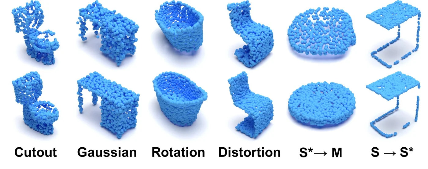 Corrupted inputs (top) and the same point clouds after CloudFixer (bottom) for four ModelNet40-C corruptions and two PointDA-10 shifts. Rotation and noise are largely undone, while the missing region from cutout stays missing. Figure from the paper.
The cost plot puts the speed claim in one picture: averaged over all ModelNet40-C corruptions, CloudFixer adapts a sample in 0.93 s at 78.4% accuracy, while DDA needs 23.6 s and MEMO is fast but no better than the unadapted model.
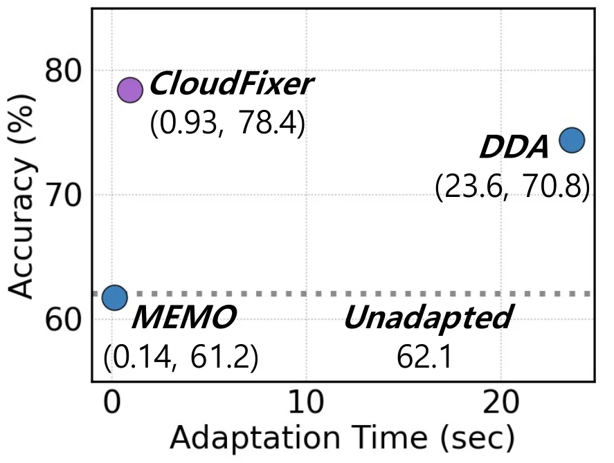 Average adaptation time per sample against accuracy on ModelNet40-C for the per-sample episodic methods. CloudFixer is about 25 times faster than DDA and more accurate. Figure from the paper.
Across backbones (Point2Vec, PointMAE, PointMLP, PointNeXt, mild setting), CloudFixer-O is the best or tied-best everywhere. Plain CloudFixer is a little below TENT with batch size 64 on three of the four backbones (it is above TENT on PointMAE), which is not surprising since TENT is strong in this easy setting.
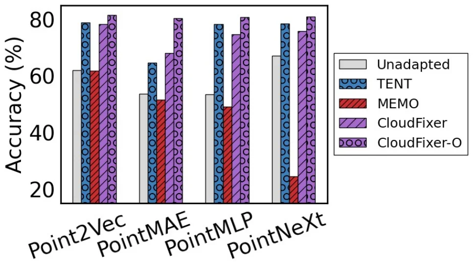 Average ModelNet40-C accuracy for four classifier backbones. CloudFixer-O is at or near the top for all of them; MEMO falls well below the unadapted model on PointNeXt. Figure from the paper.
Limitations
- Occlusion. The authors say this themselves. The diffusion model works on normalized point clouds, so a heavily occluded shape gets rescaled and shifted. Recovering it would need large point movements, which the regularizer suppresses. In Table 1, OC accuracy is 41.00 versus 41.09 unadapted.
- Small losses on density corruptions. With batch size 1, DI (90.03 to 87.32) and DD (86.51 to 80.27) drop slightly below the unadapted model.
- Per-sample cost. Each sample needs 30 optimization steps with one diffusion forward pass each, which is about 0.93 s. That is much faster than DDA but still far from a single classifier pass. Voting multiplies the work by \(K\).
- A source diffusion model is required. A Point-E model is trained for 5000 epochs on each source dataset. So the method assumes access to source data, or to a diffusion model trained on it, before deployment.
- CloudFixer-O needs more. It needs reasonably large i.i.d. batches and extra backward passes through the classifier. In the batch-size-1 PointMAE setting it uses 48 transformations per instance.
- Narrow sensitivity check. The hyperparameter sensitivity study covers only one corruption (impulse noise).