Abstract
Test-time prompt tuning (TPT) adapts CLIP’s text prompt on each test image by minimizing the entropy of predictions over augmented views. This raises accuracy but makes the model overconfident. C-TPT and O-TPT fix part of this by spreading the class text features apart (larger dispersion, or orthogonality). These diversity-based methods work, but it is not clear why, and the authors show cases where calibration is good even when text feature dispersion is low.
The paper looks at the modality gap instead. In CLIP, the gap between image and text features is concentrated in one dominant dimension per modality, and that dimension has a large effect on the logits. Replacing the text-dominant dimension with its mean lowers ECE for both zero-shot CLIP and TPT. D-TPT turns this into a loss: it pushes each class text feature, seen as a distribution over its dimensions, toward uniform, so that no single dimension dominates.
Motivation
C-TPT and O-TPT rest on an empirical link: the more the class text features are spread out (higher average text feature dispersion, ATFD), the lower the ECE. The paper’s opening plot questions that link. Zero-shot CLIP and C-TPT sit at high ATFD, TPT sits at low ATFD with high ECE, but D-TPT reaches a low ECE while its ATFD is about as low as TPT’s. So dispersion cannot be the whole story, and the authors look for another factor that controls confidence.
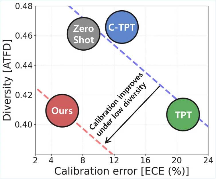 Text feature diversity (ATFD) against ECE for zero-shot CLIP, TPT, C-TPT and D-TPT. Along the blue line more diversity means lower ECE, but D-TPT (“Ours”) is calibrated at roughly TPT’s diversity, so diversity alone does not explain calibration. Figure from the paper.
Their candidate is the modality gap. Plotting the raw feature values per dimension shows that CLIP text features share one dimension (index 362) whose value is around 0.8 for every class, and image features have their own spike at a different index (442). Because these spikes are shared across classes, they carry the gap between the two modalities rather than class information, yet they dominate the dot product that forms the logits. Masking the text-dominant dimension changes predictions far more than any other dimension, and replacing it with its mean already lowers TPT’s ECE (12.34% to 10.84%) at almost the same accuracy. That pilot result is the key insight: weakening the dominant text dimension calibrates TPT without having to spread classes apart.
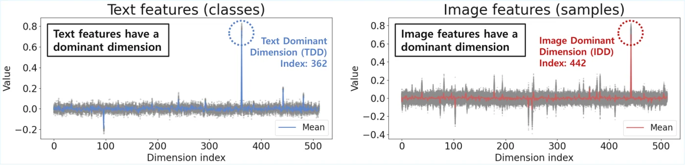 Feature value per dimension for CLIP text features (left, all classes) and image features (right, all samples). Each modality has one dominant dimension that stands far above the rest and is shared by all classes or samples. Figure from the paper.
Method
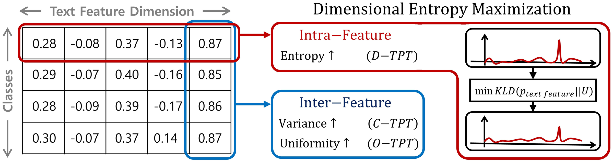 Rows are class text features, columns are feature dimensions. C-TPT and O-TPT act across classes (inter-feature). D-TPT acts within each text feature (intra-feature) and minimizes its KL divergence to a uniform distribution, which flattens the dominant dimension. Figure from the paper.
Base: TPT
For an image \(x_i\) with feature \(v_i\) and class text features \(t_c\) from the prompt “a photo of a [class]”, CLIP predicts
\[p_{i,c}=\frac{\exp(\tau\cdot\cos(t_{c},v_{i}))}{\sum_{k=1}^{C}\exp(\tau\cdot\cos(t_{k},v_{i}))}.\]TPT makes \(N-1\) augmented views of the test image (64 inputs in total), keeps the confident ones, and minimizes their entropy:
\[\mathcal{L}_{tpt}=\frac{1}{\rho N}\sum_{i=1}^{N}\mathbb{I}[H(p_{i})<\rho]\,H(p_{i}).\]Only the prompt tokens are updated. After predicting on the test sample, the prompt is reset.
Dominant dimensions (left side of the figure)
The table in the figure shows the pattern: one column (the last one) has a large value for every class. The authors call this the text-dominant dimension (TDD), and the matching one in image features the image-dominant dimension (IDD). They measure the sensitivity of each dimension \(m\) as the KL divergence between the prediction with that dimension masked, \(p_m\), and the original prediction \(q\):
\[s_{m}=KLD(p_{m}\,\|\,q).\]The dominant dimensions have by far the highest sensitivity. Replacing TDD with its class-wise mean drops the mean ECE of TPT over eight datasets from 12.34% to 10.84%, with accuracy almost unchanged (62.26% to 62.19%). Replacing IDD instead makes ECE worse (16.97%).
Dimensional entropy maximization (right side of the figure)
To reduce the weight of the dominant dimension without hand-picking it, D-TPT applies a softmax over the dimensions of each normalized text feature \(\bar{t}_c\) and pulls that distribution toward uniform \(U\):
\[\mathcal{L}_{DEM}=\frac{1}{C}\sum_{c=1}^{C}KLD(\sigma(\bar{t}_{c})\,\|\,U).\]Minimizing this KL is the same as maximizing the entropy of \(\sigma(\bar{t}_c)\). The total loss is
\[\mathcal{L}_{D\text{-}TPT}=\mathcal{L}_{TPT}+\lambda\cdot\mathcal{L}_{DEM},\]with \(\lambda=10^{5}\) fixed for all datasets and both backbones.
How it differs from C-TPT and O-TPT
The bottom-left box of the figure is the inter-feature view. C-TPT adds \(\frac{1}{C}\sum_{c}\lVert\bar{t}_{c}-\frac{1}{C}\sum_{j}\bar{t}_{j}\rVert_{2}\) to push class features away from their centroid. O-TPT adds \(\lVert TT^{\top}-I_{C}\rVert^{2}_{2}\) to make them orthogonal. Both compare features across classes. D-TPT only looks at the shape of each feature on its own.
The paper gives a geometric argument on the unit hypersphere. TPT moves the top-1 text feature toward the image along the tangent direction and pushes the others away, which widens the logit range and causes overconfidence. D-TPT instead spreads mass to the other dimensions, which the authors describe as the binormal direction. Empirically it keeps a similar text dispersion (ATFD) to TPT but gives a smaller logit range and a smaller modality gap, and a smaller logit range means lower softmax confidence. The authors note this is a geometric intuition, not a full theory.
Main Experiments
Setup: CLIP ViT-B/16 and RN50, single-sample TPT with 63 augmentations, AdamW with lr 0.005. Numbers are averages over 11 fine-grained datasets (Table 1) or 4 ImageNet variants, A/V2/R/Sketch (Table 2), each as the mean of 3 seeds. Standard deviations are left out here. ECE in %, AURC in \(\times 10^{3}\), lower is better for both. The paper also reports AECE and MCE, which are omitted.
Fine-grained classification (11 datasets, average)
| Method | ViT-B/16 Acc. | ViT-B/16 ECE | ViT-B/16 AURC | RN50 Acc. | RN50 ECE | RN50 AURC |
|---|---|---|---|---|---|---|
| Zero-shot | 63.84 | 4.25 | 184.28 | 56.05 | 5.25 | 254.15 |
| TPT | 65.09 | 11.42 | 185.64 | 58.07 | 11.27 | 251.15 |
| C-TPT | 64.46 | 4.97 | 187.50 | 57.57 | 6.20 | 243.87 |
| O-TPT | 63.98 | 4.78 | 187.25 | 57.36 | 5.63 | 244.96 |
| D-TPT | 64.72 | 4.18 | 181.67 | 57.13 | 5.91 | 245.27 |
Natural distribution shifts (ImageNet-A/V2/R/Sketch, average)
| Method | ViT-B/16 Acc. | ViT-B/16 ECE | ViT-B/16 AURC | RN50 Acc. | RN50 ECE | RN50 AURC |
|---|---|---|---|---|---|---|
| Zero-shot | 57.19 | 4.93 | 216.23 | 40.66 | 7.19 | 395.77 |
| TPT | 60.24 | 11.77 | 211.24 | 43.35 | 17.06 | 383.07 |
| C-TPT | 58.33 | 5.42 | 210.52 | 41.76 | 8.99 | 390.19 |
| O-TPT | 58.48 | 5.14 | 209.91 | 41.74 | 8.97 | 390.24 |
| D-TPT | 57.87 | 3.83 | 211.31 | 42.92 | 8.05 | 379.73 |
(Zero-shot ECE is excluded from the bold marks; on fine-grained RN50 zero-shot ECE, 5.25, is lower than every tuned method.)
With ViT-B/16, D-TPT has the lowest ECE among the tuned methods on both benchmarks, and on the fine-grained sets it also beats O-TPT in accuracy (64.72 vs. 63.98). On RN50 fine-grained it sits between C-TPT and O-TPT and is not the best, which the authors state. All calibration methods, including D-TPT, still give back part of TPT’s accuracy gain.
The reliability diagrams show where the ECE gain comes from. On DTD, TPT’s confidence histogram piles up near 1.0 with large gaps in every bin, while D-TPT’s bars track the diagonal. On Stanford Cars, the failure case, zero-shot CLIP is already nearly calibrated and all tuned methods are close, so D-TPT has no margin to win.
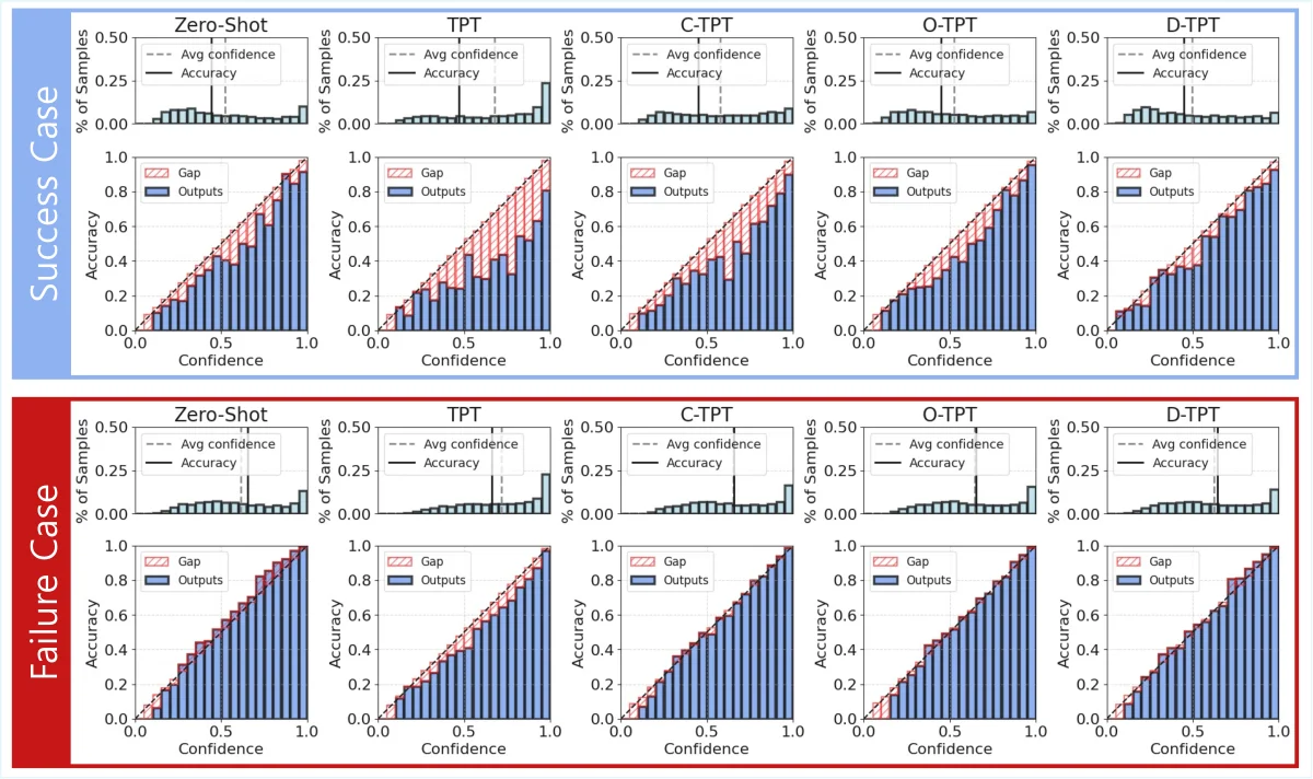 Confidence histograms and reliability diagrams for zero-shot CLIP, TPT, C-TPT, O-TPT and D-TPT on DTD (success case, top) and Stanford Cars (failure case, bottom). Red hatched areas are the accuracy-confidence gap; on DTD TPT’s gap is large and D-TPT’s is the smallest. Figure from the paper.
The Pareto plots sweep the weight \(\lambda\) of each regularizer. On DTD, D-TPT reaches the lowest ECE of the three (about 5.4%) at an accuracy similar to O-TPT at its lowest ECE, and on Flowers102 it sits at clearly higher accuracy (about 72% vs. 69 to 70%) with ECE as low as O-TPT’s.
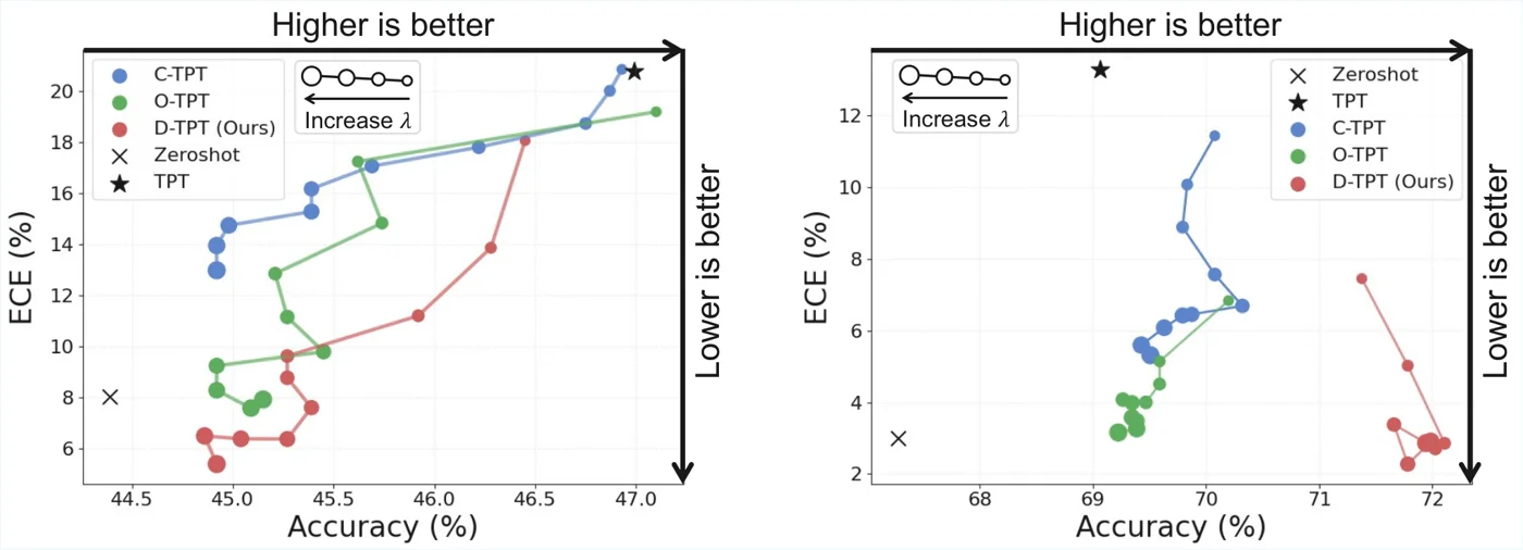 Accuracy-ECE trade-off as \(\lambda\) increases (larger markers) for C-TPT, O-TPT and D-TPT on DTD (left) and Flowers102 (right); lower right is better. D-TPT reaches low ECE while losing less accuracy than the inter-feature methods. Figure from the paper.
Limitations
- Theory is partial (stated by the authors). The geometric argument considers text features moving relative to a single image feature, while TPT actually uses many augmented views. The link between the modality gap and calibration is not proven.
- Not best on RN50 fine-grained. O-TPT has lower ECE and C-TPT lower AURC there, and D-TPT has the lowest accuracy of the three.
- Accuracy trade-off remains. On the ImageNet variants with ViT-B/16, D-TPT is 0.61 points below O-TPT and 2.37 points below TPT in accuracy.
- MCE not consistently better. O-TPT has the best MCE on fine-grained ViT-B/16, so the gain is not uniform across calibration metrics.
- Very large, fixed \(\lambda\). \(\lambda=10^{5}\) reflects the small scale of the KL term. It is fixed across settings, and its effect is shown only with Pareto plots on DTD and Flowers102.
- Prompt initialization matters. With a CoOp-trained prompt as initialization, D-TPT still has the lowest ECE among the tuned methods (6.96), but its accuracy (63.20) and AURC (195.41) are the worst of the four tuned methods in that setting.
- CLIP-specific premise. The method relies on the observation of one dominant dimension in CLIP features. Whether other contrastive VLMs share this property is not tested.