Abstract
Test-time prompt tuning (TPT) adapts CLIP’s text prompt to each test image with an entropy minimisation (EM) loss. It raises accuracy but makes predictions overconfident. C-TPT and O-TPT add a regulariser that spreads the class text features apart. This lowers calibration error but often costs accuracy, and it does not explain why spreading features should help calibration.
This paper gives one explanation. Because TPT resets the prompt for every test sample and takes a single step, the regulariser’s gradient is a fixed offset. Regularised TPT then looks like sharpness-aware minimisation (SAM): the EM gradient is computed at a perturbed point and applied at another. The authors show that flatter minima go with lower calibration error. Their method, Flatness-aware Prompt Pretraining (FPP), drops the regulariser and instead pretrains the initial prompt, without any images, so that it already sits in a flat region. Existing TPT pipelines only need to swap their initial prompt.
Motivation
C-TPT and O-TPT were designed as geometric constraints on the text features, and they work, but the papers do not say what the constraint does to the prompt itself. FPP looks at the prompt’s loss landscape instead. Measuring the sharpness of the entropy loss around each adapted prompt, the authors find a clean ordering on the fine-grained average: TPT has the sharpest minima and the highest ECE (11.67%), C-TPT is flatter with lower ECE, and O-TPT is flatter still with lower ECE again. Sharpness and ECE fall together, which suggests the regularizers help calibration by pushing the prompt toward flat minima, the same property that sharpness-aware training targets for generalization.
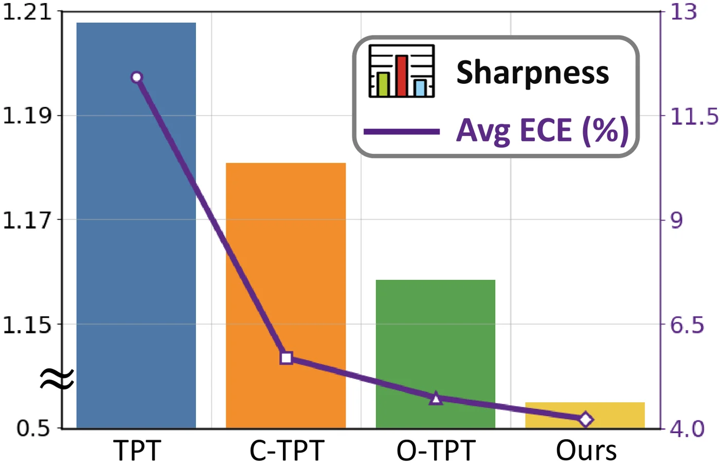 Average sharpness of the adapted prompt (bars, left axis, broken at the bottom) and average ECE (line, right axis) on the fine-grained datasets. Adding C-TPT’s or O-TPT’s regularizer lowers both, and FPP (“Ours”) is the flattest with the lowest ECE. Figure from the paper.
The authors then point out two problems with getting flatness through those regularizers. Constraining the output features directly often costs accuracy, and with a single TPT step the prompt cannot travel far enough to find a flatter region; taking more steps risks becoming overconfident on wrong predictions. The insight behind FPP is to move the search for flatness out of test time: if the starting prompt already sits in a flat region, the usual one-step entropy update will end in a flat minimum without any regularizer.
Method
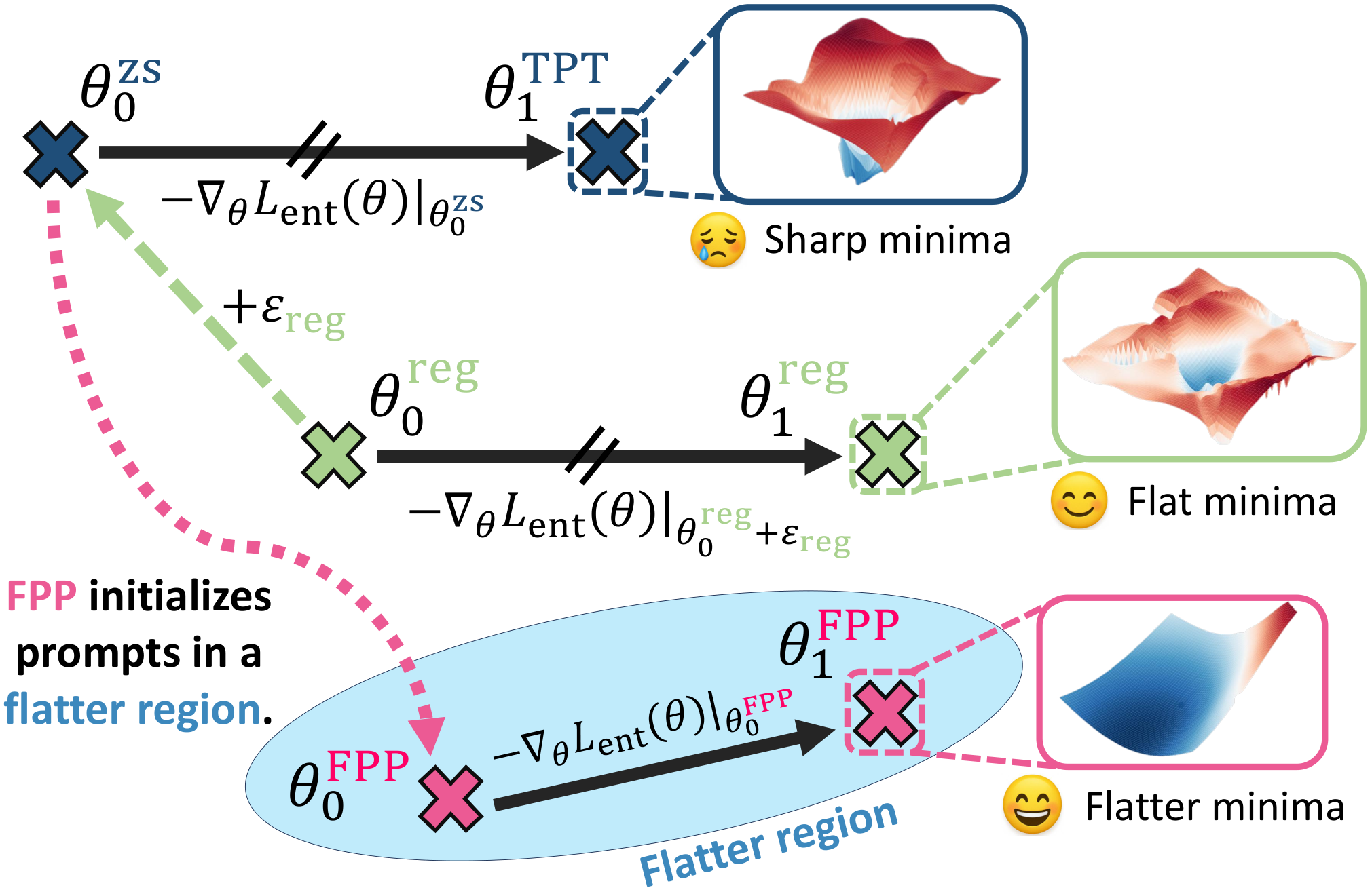 Top: plain TPT takes one EM step from the zero-shot prompt and lands in a sharp minimum. Middle: regularised TPT is equivalent to starting from a shifted prompt and computing the EM gradient at a perturbed point, which leads to a flatter minimum. Bottom: FPP pretrains the initial prompt inside a flatter region, so a plain EM step lands in an even flatter minimum. Figure from the paper.
Regularised TPT as SAM (top and middle rows)
TPT optimises a prompt \(\theta\) with the entropy of the prediction averaged over confident augmented views \(V\), \(L_{\text{ent}}(\theta, V)\). C-TPT and O-TPT add \(\lambda L_{\text{reg}}(\theta)\), where \(L_{\text{reg}}\) depends only on the text features \(f_T(C;\theta)\) of the fixed class names \(C\):
\[L_{\text{reg}}^{\text{C-TPT}} = -\frac{1}{K}\sum_{k=1}^{K}\|t_k - \mu\|_2, \qquad L_{\text{reg}}^{\text{O-TPT}} = \|TT^\top - I_K\|_2^2 .\]| Every test sample starts from the same prompt \(\theta_0^{\text{zs}}\), so $$\varepsilon_{\text{reg}} = \lambda \nabla_\theta L_{\text{reg}}\big | _{\theta_0^{\text{zs}}}$$ is the same constant for all samples. With unit learning rate, one step is |
| with \(\theta_0^{\text{reg}} := \theta_0^{\text{zs}} - \varepsilon_{\text{reg}}\). So regularised TPT is plain TPT from a shifted start, with the gradient taken at a perturbed point. Theorem 1 links the two losses: for an image feature drawn uniformly from the unit sphere, the expected EM loss is an affine function of \(L_{\text{reg}}\) up to \(O(D^{-3/2})\). The perturbed point therefore tends to have higher EM loss, which is the same pattern as SAM’s update $$w_{t+1} = w_t - \eta \nabla_w L(w, v)\big | _{w_t + \hat{\varepsilon}_t}$$. Empirically, C-TPT and O-TPT reach lower sharpness than TPT, and when prompts are grouped by sharpness, flatter groups have lower ECE. |
Flatness-aware prompt pretraining (bottom row)
FPP moves the search for flatness to before test time. It learns a new initial prompt \(\theta\) with two losses. The flatness loss asks the text features to stay the same when both the class-name embeddings and the prompt are perturbed by small Gaussian noise \(\varepsilon_1, \varepsilon_2\):
\[\mathcal{L}_{\text{flat}} = \operatorname{dist}_{\cos}\big(f_T(C + \varepsilon_1;\, \theta + \varepsilon_2),\; f_T(C;\, \theta)\big).\]Lower output sensitivity gives lower sharpness for any differentiable loss on top of the text features (proved in the appendix). On its own, this loss destroys the zero-shot features, so an alignment loss keeps the new text features close to those of the original prompt:
\[\mathcal{L}_{\text{align}} = \operatorname{dist}_{L2}\big(f_T(C;\, \theta),\; f_T(C;\, \theta_0^{\text{zs}})\big), \qquad \mathcal{L}_{\text{FPP}} = \mathcal{L}_{\text{align}} + \lambda\, \mathcal{L}_{\text{flat}} .\]The weight is \(\lambda = \gamma_1 + \gamma_2 / K\) with \(\gamma_1 = 1.0\) and \(\gamma_2 = 0.15\), which lowers the flatness weight for many classes. Pretraining runs 1K AdamW iterations with lr 0.01, and the noise variances are 0.02 for \(\varepsilon_1\) and 0.005 for \(\varepsilon_2\). Both losses use only the prompt and the class names, so no images are needed. At test time the TPT procedure is unchanged: only \(\theta_0^{\text{zs}}\) is replaced by the pretrained prompt, and no regulariser is added.
Main Experiments
Setup: CLIP ViT-B/16, hard prompt “a photo of a”, standard TPT test-time settings as in C-TPT and O-TPT. Metrics are top-1 accuracy (%), ECE (%), and SCE (static calibration error). FPP here means TPT started from the FPP prompt. The table shows only the average columns of the paper’s Table 1 (10 fine-grained datasets: Aircraft, Caltech, Cars, DTD, EuroSAT, Flowers, Food, Pets, SUN, UCF) and Table 4 (OOD average over ImageNet-A, -V2, -R, -Sketch), plus the ImageNet column of Table 4.
| Method | Fine-grained Acc | ECE | SCE | ImageNet Acc | ECE | OOD Acc | ECE | SCE |
|---|---|---|---|---|---|---|---|---|
| CLIP | 63.41 | 4.67 | 1.06 | 66.7 | 2.12 | 57.18 | 5.04 | 0.15 |
| TPT | 64.62 | 11.67 | 1.15 | 69.0 | 10.6 | 59.95 | 11.99 | 0.14 |
| C-TPT | 64.48 | 5.32 | 1.11 | 68.5 | 3.15 | 59.55 | 5.82 | 0.14 |
| O-TPT | 64.12 | 4.46 | 1.15 | 67.3 | 1.97 | 57.82 | 4.88 | 0.15 |
| FPP | 65.37 | 4.13 | 0.96 | 67.8 | 2.97 | 59.53 | 4.63 | 0.12 |
With prompts initialised from released CoOp and MaPLe checkpoints (paper’s Table 2, fine-grained average):
| Method | Acc | ECE |
|---|---|---|
| CoOp+TPT | 63.91 | 18.36 |
| CoOp+C-TPT | 63.56 | 10.04 |
| CoOp+O-TPT | 63.29 | 7.91 |
| CoOp+FPP | 64.78 | 5.67 |
| MaPLe+TPT | 65.75 | 6.94 |
| MaPLe+O-TPT | 65.05 | 4.11 |
| MaPLe+FPP | 67.01 | 4.07 |
On the fine-grained average, FPP is the only method that beats TPT in accuracy while also having the lowest ECE and SCE. On the OOD sets it keeps most of TPT’s accuracy (59.53 vs. 59.95) with lower ECE than O-TPT, though the shift experiments use a fixed \(\lambda = 1.25\). The ablation shows both parts are needed: alignment alone gives 7.05 ECE, flatness alone collapses zero-shot accuracy to 4.65%, and the full loss gives 4.13. Applying SAM or ASAM directly inside TPT also lowers ECE, but SAM drops accuracy to 61.59.
The sharpness-group analysis is the paper’s direct check that flatness tracks calibration. For each test sample a prompt is adapted, the prompts are split into thirds by sharpness, and ECE is computed per group and averaged over the fine-grained datasets. For TPT, C-TPT, O-TPT and FPP alike, the flattest third has the lowest ECE. This is a correlation across groups, not a causal test.
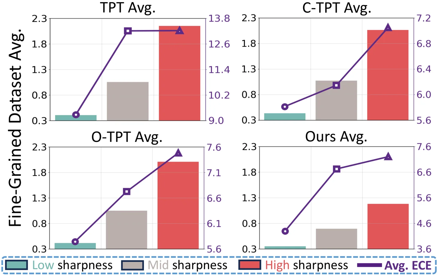 Prompts split into low, mid and high sharpness thirds (bars) with the average ECE of each group (line), for TPT, C-TPT, O-TPT and FPP on the fine-grained datasets. In every method, flatter groups are better calibrated. Figure from the paper.
The reliability diagrams compare O-TPT and FPP on three datasets. The largest change is on EuroSAT, where O-TPT’s mid-confidence bins are badly overconfident (ECE 12.98) and FPP’s bars follow the diagonal (5.19). On DTD the two are close (7.88 vs. 7.52), and on SUN397 FPP removes O-TPT’s underconfidence in the low bins.
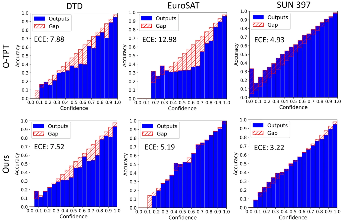 Reliability diagrams of O-TPT (top) and FPP (bottom) on DTD, EuroSAT and SUN397, with the ECE of each. FPP corrects both overconfidence (EuroSAT) and underconfidence (SUN397), while DTD barely changes. Figure from the paper.
Limitations
- EuroSAT drives the fine-grained average. FPP reaches 50.66% on EuroSAT against 42.4% for TPT. Averaging the paper’s Table 1 over the other nine datasets gives about 67.0% for FPP and 67.1% for TPT, and an ECE of about 4.0 for FPP against 3.5 for O-TPT. The overall lead depends on that one dataset.
- Mixed per-dataset calibration. FPP’s ECE is clearly worse than O-TPT on Aircraft (7.26 vs. 3.68), Caltech (5.85 vs. 3.80), ImageNet (2.97 vs. 1.97) and ImageNet-R (7.07 vs. 1.46).
- Accuracy under shift. On the OOD average FPP is slightly below TPT and C-TPT in accuracy, and on ImageNet it is below both.
- Theory under strong assumptions. The SAM view assumes a single step with unit learning rate and no momentum. Theorem 1 assumes image features uniform on the sphere and holds up to an \(O(D^{-3/2})\) term. The link between flatness and calibration is shown by correlation across sharpness groups, not proved.
- Per-task pretraining. A new prompt is pretrained for each class set, which takes about 10 minutes for SUN397. Table 6 shows ImageNet class names or Gaussian noise as stand-ins work nearly as well, which softens this.
- Single backbone. All main results use CLIP ViT-B/16. The DynaPrompt baseline is a replication that falls below the original paper’s accuracy (64.22 vs. 65.43).