Abstract
Point cloud classifiers trained on clean data lose a lot of accuracy on corrupted test data such as background clutter, occlusion, or LiDAR-style sampling. Test-time adaptation (TTA) tries to fix this online, using only the unlabeled test batches. Existing 3D TTA methods mostly work in the spatial domain. MATE needs an extra reconstruction task during source training. BFTT3D needs feature prototypes from source data. CloudFixer and 3DD-TTA need a diffusion model trained on source data. And methods that learn a per-point offset \(\Delta P \in R^{N\times 3}\) face a high-dimensional problem that is hard to solve from a few streaming test samples.
GSDTTA moves the adaptation to the graph spectral domain. Each test point cloud becomes a kNN graph, is transformed with the Graph Fourier Transform (GFT), and only the lowest \(M=100\) frequency coefficients (about 10% of them) get a learnable offset. The inverse GFT turns this offset into a smooth, global point shift. Pseudo-labels for the optimisation mix the model’s deep features with Laplacian eigenmap features, which the authors argue are less biased toward the source domain.
Motivation
The starting point is how badly a standard classifier breaks. A DGCNN trained on clean ModelNet40 loses more than 35 points of accuracy on background, occlusion, and LiDAR corruptions, and most of that drop already happens at the lowest severity level.
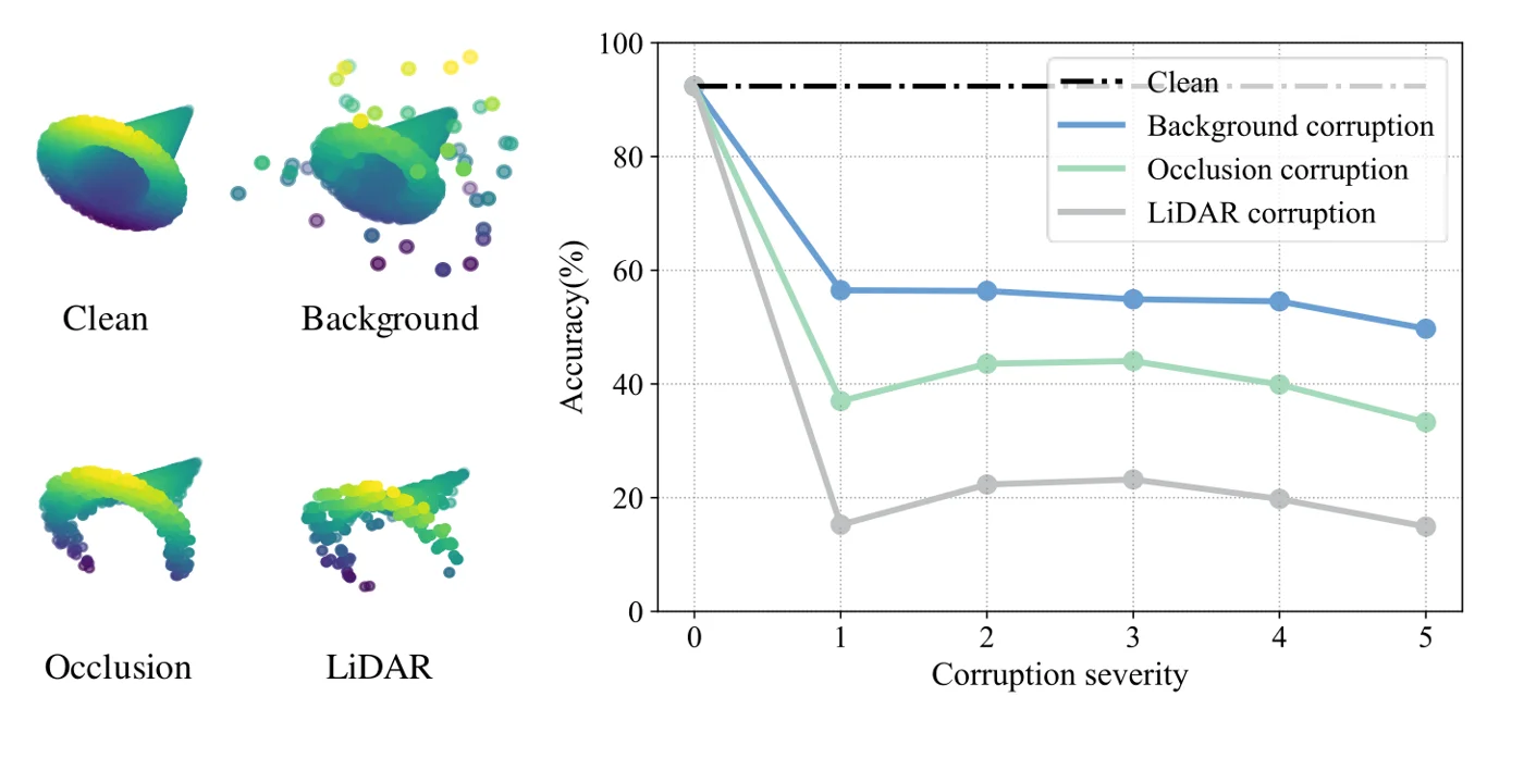 Left: a clean shape and its background, occlusion, and LiDAR versions. Right: DGCNN accuracy drops from about 92% to roughly 50%, 35%, and 15% as severity grows, with most of the loss at level 1. Figure from the paper.
The authors then point at what existing 3D TTA methods have in common: they all work in the spatial domain. MATE solves masked patch reconstruction, and CloudFixer and 3DD-TTA learn a per-point transformation \(\Delta P \in R^{N\times 3}\) with \(N\) often above 1024. CloudFixer and 3DD-TTA also need a diffusion model trained on source data. With only a few streaming test samples, such a high-dimensional problem is hard to optimise.
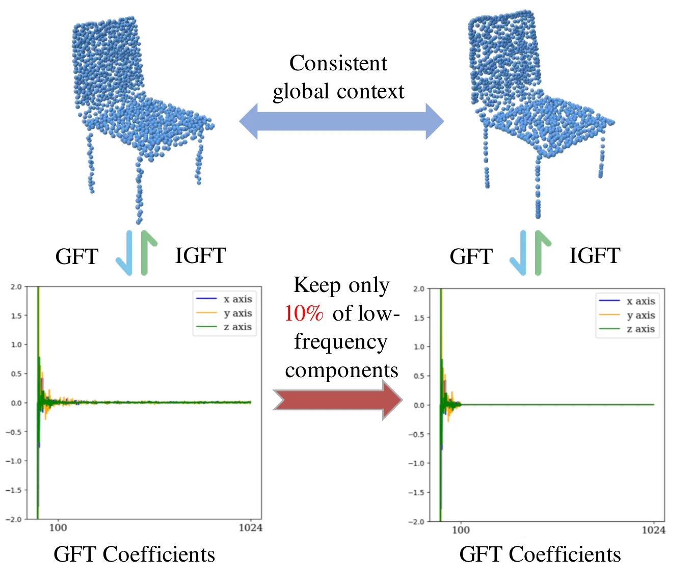 GFT coefficients of a chair (left) are almost all near zero after the first ~100. Keeping only those lowest 10% and applying the inverse GFT (right) gives back the same global shape. Figure from the paper.
Two observations about the graph spectral domain give the key insight. First, energy compaction: about 95% of a chair’s spectral energy sits in roughly the lowest 100 coefficients, so editing only those controls the global shape with about 90% fewer parameters than editing points directly. Second, Laplacian eigenmaps are isometry-invariant shape descriptors that do not depend on any training domain. Deep features carry source bias, especially early in adaptation, so the eigenmaps can serve as a second, unbiased opinion when building pseudo-labels.
Method
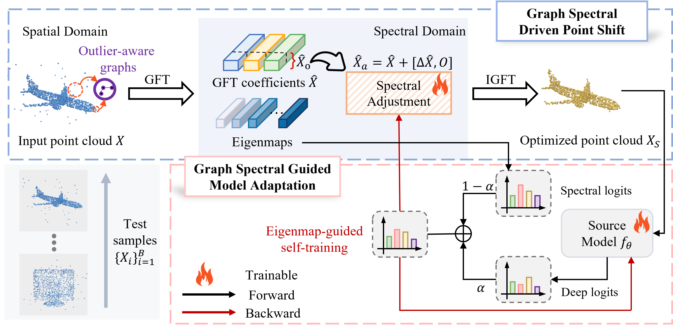 The GSDTTA pipeline. The top half (GSDPS) shifts the input point cloud through the spectral domain. The bottom half (GSGMA) updates the model. Both are trained with eigenmap-guided pseudo-labels. Figure from the paper.
The method has two modules that take turns on each test batch \(\{X_i\}_{i=1}^{B}\): Graph Spectral Driven Point Shift (GSDPS) adapts the input, and Graph Spectral Guided Model Adaptation (GSGMA) adapts the model \(f_\theta\).
Outlier-aware graph
For a point cloud \(X \in \mathbb{R}^{N\times 3}\), edges connect each point to its \(k\) nearest neighbours and are weighted with an RBF kernel:
\[w_{ij} = \exp\left(-\frac{d^2(x_i, x_j)}{2\delta^2}\right), \qquad A_{ij} = w_{ij}\cdot \mathbb{I}(x_j \in \mathcal{N}(x_i)).\]Spectral analysis is sensitive to outliers. Outliers sit far from other points, so their degree (sum of edge weights) is low. GSDTTA drops vertices whose degree is below a threshold \(\tau\):
\[A^o_{ij} = w_{ij}\cdot \mathbb{I}(x_j \in \mathcal{N}(x_i)) \cdot \mathbb{I}\Big(\sum_{j=1}^{N} A_{ij} > \tau\Big), \qquad \tau = \frac{\gamma}{Nk}\sum_{i=1}^{N}\sum_{j=1}^{N} A_{ij}.\]Spectral adjustment and point shift
The Laplacian \(L_o = D_o - A_o\) is eigen-decomposed as \(L_o = U_o \Lambda_o U_o^T\). The GFT of the coordinates is
\[\hat{X} = U_o^T X, \qquad \hat{X} \in \mathbb{R}^{N\times 3}.\]A learnable offset \(\Delta\hat{X} \in R^{M\times 3}\) with \(M \ll N\) is added only to the low-frequency rows, and the result goes back through the inverse GFT:
\[\hat{X}_a = \hat{X} + [\Delta\hat{X}, O], \qquad X_s = U_o \hat{X}_a.\]Here \(O\) is an \((N-M)\times 3\) zero matrix. The motivation is energy compaction: for a chair shape, about 95% of the spectral energy is in the low frequencies, and the lowest 10% of coefficients are enough to rebuild the global shape. So the optimisation has \(M\times 3 = 300\) parameters per point cloud instead of \(N\times 3\).
Eigenmap-guided self-training
The eigenvectors also give a shape descriptor. Dropping the eigenvector for \(\lambda_1 = 0\) and keeping \(m\) others embeds each node as \(E(v_i) = [u_1(v_i), \dots, u_m(v_i)]\). Max-pooling over nodes gives a global spectral descriptor \(f_s\), a simplified Global Point Signature. The model’s own global feature is the deep descriptor \(f_d\).
Class centroids are built in both spaces, weighting each sample by its predicted probability:
\[q_d^c = \frac{\sum_{i=1}^{B} (f_\theta(X_i))_c\, f_d^i}{\sum_{i=1}^{B} (f_\theta(X_i))_c}, \qquad q_s^c = \frac{\sum_{i=1}^{B} (f_\theta(X_i))_c\, f_s^i}{\sum_{i=1}^{B} (f_\theta(X_i))_c}.\]The pseudo-label mixes the cosine similarity to both sets of centroids with weight \(\alpha\):
\[\hat{y}_i = \arg\max_c \left( \alpha \frac{(f_d^i)^T q_d^c}{\|f_d^i\|\|q_d^c\|} + (1-\alpha)\frac{(f_s^i)^T q_s^c}{\|f_s^i\|\|q_s^c\|} \right).\](The paper’s Eq. 16 writes \(\arg\min\). Since the terms are similarities, it is written here as picking the most similar centroid.)
What is optimised
The input step optimises only the spectral offset:
\[\arg\min_{\Delta\hat{X}} \mathcal{L}_{IA} = \mathcal{L}_{pl} + \beta_1(\mathcal{L}_{ent} + \mathcal{L}_{div}) + \beta_2 \mathcal{L}_{cd},\]where \(\mathcal{L}_{pl}\) is cross-entropy between \(f_\theta(X_s)\) and \(\hat{y}\), \(\mathcal{L}_{ent} + \mathcal{L}_{div}\) is the usual information-maximisation loss, and \(\mathcal{L}_{cd}\) is a one-directional Chamfer distance from \(X\) to \(X_s\) that keeps the shifted cloud close to the input. The model step updates \(\theta\) with the same loss minus the Chamfer term:
\[\arg\min_{\theta} \mathcal{L}_{MA} = \mathcal{L}_{pl} + \beta_3(\mathcal{L}_{ent} + \mathcal{L}_{div}).\]Per batch, GSDTTA runs 4 input steps then 1 model step, cycling for 10 steps in total (AdamW, lr 0.0001, batch size 32, \(k=10\), \(M=100\)).
Main Experiments
Backbones are DGCNN, CurveNet, and PointNeXt, trained on the clean dataset and adapted with batch size 32. The metric is classification accuracy (%), averaged over the 15 corruptions. The tables below show only the mean column of the paper’s Tables 1 and 2. 3DD-TTA is reported only with DGCNN. Baseline numbers come from the authors running each method’s published code with the same pre-trained weights.
ModelNet40-C, mean accuracy (%)
| Method | DGCNN | CurveNet | PointNeXt |
|---|---|---|---|
| Source-only | 66.51 | 71.38 | 66.99 |
| BN | 73.34 | 77.45 | 80.02 |
| PL | 75.02 | 78.56 | 80.81 |
| DUA | 73.81 | 77.41 | 80.57 |
| TENT | 75.91 | 77.88 | 81.08 |
| SHOT | 77.36 | 81.24 | 80.46 |
| BFTT3D | 65.86 | 70.95 | 68.39 |
| CloudFixer | 76.54 | 77.91 | 76.04 |
| 3DD-TTA | 71.69 | – | – |
| GSDTTA | 79.07 | 82.63 | 82.51 |
ScanObjectNN-C, mean accuracy (%)
| Method | DGCNN | CurveNet | PointNeXt |
|---|---|---|---|
| Source-only | 55.72 | 53.06 | 50.66 |
| BN | 57.15 | 57.33 | 56.68 |
| PL | 57.68 | 57.90 | 56.41 |
| DUA | 57.47 | 58.35 | 58.13 |
| TENT | 57.31 | 58.71 | 58.05 |
| SHOT | 56.32 | 58.17 | 57.06 |
| BFTT3D | 56.47 | 52.57 | 51.10 |
| CloudFixer | 60.73 | 58.96 | 59.01 |
| 3DD-TTA | 57.08 | – | – |
| GSDTTA | 61.83 | 62.59 | 60.84 |
The full per-corruption table for ModelNet40-C shows where the mean gains come from. GSDTTA is strong on background and on the shape-level corruptions (shear, rotation, distortion), while CloudFixer leads most of the noise columns and SHOT leads occlusion.
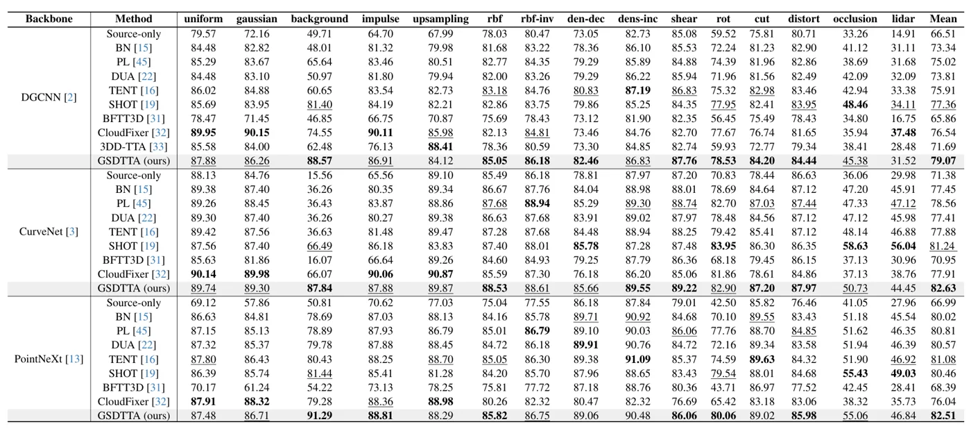 Table 1 of the paper: accuracy (%) for each of the 15 ModelNet40-C corruptions with DGCNN, CurveNet, and PointNeXt. Note the background column (88.57 for GSDTTA vs. 49.71 source-only on DGCNN) and how low occlusion and LiDAR stay for every method. Figure from the paper.
GSDTTA has the best mean on both benchmarks and all three backbones. The biggest single gain is on the background corruption (for example 88.57 vs. 49.71 source-only with DGCNN on ModelNet40-C), which the ablation ties to the outlier-aware graph: with \(\gamma=0\), background accuracy on ScanObjectNN-C drops from 69.54% to 18.24%. CloudFixer is still better on the simple noise corruptions (uniform, gaussian, impulse, upsampling) on ScanObjectNN-C, by 8.35% on average, since it uses a diffusion denoiser. In the DGCNN ablation on ScanObjectNN-C, removing the input shift costs 4.55 points, removing model adaptation costs 3.48, and replacing eigenmap-guided pseudo-labels with deep-feature-only ones costs 0.63.
To check the eigenmap idea directly, the authors compare pseudo-labels obtained from deep descriptors only, spectral descriptors only, and the eigenmap-guided mix of Eq. 16 on four corruptions.
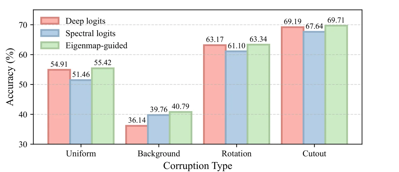 Pseudo-label accuracy from deep logits, spectral logits, and the eigenmap-guided mix on uniform, background, rotation, and cutout. Spectral logits alone are worse than deep logits except on background, but the mix is the best in all four. Figure from the paper.
Limitations
- Scalability (stated by the authors). Global spectral operations are expensive, which limits use on large point clouds. They suggest segmentation and multi-scale local spectral analysis as future work.
- Eigen-decomposition per sample. Every test point cloud needs its own Laplacian eigen-decomposition. A full decomposition of an \(N\times N\) matrix scales as \(O(N^3)\), and even computing a subset of eigenvectors adds cost that grows with \(N\).
- Many optimisation steps per batch. Each batch gets 10 backward-pass steps (8 on the input, 2 on the model). The main paper does not report runtime or memory, so the latency cost versus TENT or BN is not clear.
- Batch assumptions. The class centroids and the diversity loss are computed over the batch (size 32 in all experiments). Behaviour with small batches or single-sample streams is not shown in the main paper.
- Hard corruptions remain hard. Occlusion and LiDAR stay low for every method, for example 45.38 and 31.52 for GSDTTA with DGCNN on ModelNet40-C, and around 10% on ScanObjectNN-C.
- Many hyperparameters. \(k\), \(\delta\), \(\gamma\), \(M\), \(\alpha\), \(\beta_1\), \(\beta_2\), \(\beta_3\) are fixed by hand. Sensitivity is shown only for the three \(\beta\) weights, on one corruption (shear) with one backbone.