Abstract
Most test-time adaptation (TTA) recipes come from CNNs with Batch Normalization (BN). They re-estimate batch statistics or update BN’s affine parameters with entropy minimization. Point-cloud classifiers like Point-MAE are Transformers, and Transformers use Layer Normalization (LN). LN normalizes each token across its features and never looks at the batch axis, so BN-style fixes do not transfer cleanly. Existing point-cloud TTA methods also have practical costs: TENT needs backpropagation, MATE needs a special pretraining objective, BFTT3D needs source prototypes, and multi-sampling methods need many extra passes.
The paper analyzes LN from the batch (domain) point of view. It shows that LN’s pre-affine output is already close to zero mean and unit variance per feature across the batch when the feature dimension and batch size are large. So there is no need to re-standardize. The only thing worth adjusting is the post-affine mean and gain. LN-TTA does this with one forward pass, no gradients, and no source data, using a prototype read from the pretrained [cls] token.
Motivation
The authors trace the weak results of existing point-cloud TTA to a mismatch in normalization. Recipes like BN re-estimation and TENT assume BN, which normalizes each feature across the batch, so every downstream weight sees steady per-feature statistics, and that is exactly the lever these methods pull. Point-MAE and other point Transformers use LN, which normalizes each token across its own features and never touches the batch axis. So it is not obvious what a BN-style fix should even change in an LN model.
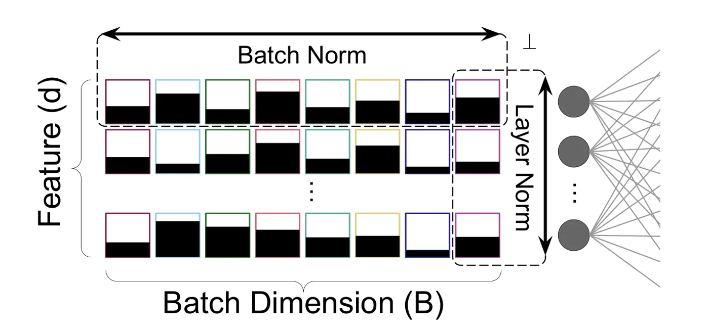 BN works on one feature across the batch (horizontal box), while LN works on one sample across its features (vertical box). The two methods give different handles for test-time adaptation. Figure from the paper.
The practical gaps add to this. TENT underperforms on point clouds and needs backpropagation, MATE ties adaptation to a special MAE pretraining, multi-sampling methods need many extra passes, and BFTT3D needs class-level source prototypes at test time. The paper’s answer is to look at LN from the batch side. LN already removes per-token shift and scale exactly, and as \(d\) and \(B\) grow the per-feature batch marginals of its pre-affine output approach \((0, 1)\). So LN already does the stabilizing that BN-style TTA tries to add, and re-standardizing is unnecessary or even harmful. What is left to fix is the post-affine mean and gain.
Method
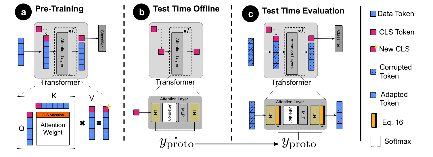 (a) During pretraining the [cls] token aggregates information from the data tokens. (b) Offline, a forward pass with only the [cls] token records a prototype \(y_{\text{proto}}\) at every LN layer. (c) At test time, each LN output is recoloured with Eq. 16 using the stored prototype. Figure 2 from the paper.
Background: LN as projection plus rescaling
For a token \(x_t \in \mathbb{R}^d\), LN is
\[\mathrm{LN}(x_t) = \gamma \odot \frac{x_t - \mu_d(x_t)\mathbf{1}}{\sqrt{\sigma_d^2(x_t) + \varepsilon}} + \beta .\]The paper splits this into a pre-affine map and a per-feature affine. With \(u = \mathbf{1}/\sqrt{d}\) and \(C = I - uu^\top\) (which removes the token mean),
\[\widehat{\mathrm{LN}}(x_t) = \sqrt{d}\,\frac{C x_t}{\sqrt{\|C x_t\|^2 + d\varepsilon}}, \qquad \mathrm{LN}(x_t) = \Gamma\,\widehat{\mathrm{LN}}(x_t) + \beta, \quad \Gamma = \mathrm{diag}(\gamma).\]So LN first projects onto the mean-zero hyperplane \(H\), then normalizes the radius, then applies \((\gamma, \beta)\). The pre-affine part is invariant to adding a constant to all features and (for \(\varepsilon = 0\)) to global rescaling.
Theory: LN already standardizes across the batch
Per token, \(\widehat{\mathrm{LN}}\) gives exactly zero mean and unit second moment across features (Proposition 1, \(\varepsilon = 0\)). The key result is about the batch axis. Fix a token \(t\) and feature \(j\), and let \(H_{b,t} = \widehat{\mathrm{LN}}(x_{b,t})\). Theorem 1 says that as \(d \to \infty\) and \(B = B(d) \to \infty\),
\[\bar H_{j,B} \xrightarrow{P} 0, \qquad S^2_{j,B} \xrightarrow{P} 1,\]where \(\bar H_{j,B}\) and \(S^2_{j,B}\) are the batch mean and variance of feature \(j\). After the affine, the per-feature batch limits become \((\beta_j, \gamma_j^2)\). In words: LN does the BN job implicitly, and the post-affine mean and scale are controlled only by \((\gamma, \beta)\). The design rule is to keep the pre-affine step and adjust only the affine.
(a)-(b) A prototype from the [cls] token
If source post-affine moments were available, one could match them per feature (Eq. 13-14 in the paper). In the source-free setting they are not. The authors note that the [cls] token aggregates domain information during pretraining. So, with the model frozen, they run one forward pass with only the [cls] token (attention over a length-1 sequence is the identity on \(V\)) and record, at each LN layer,
\[y_{\text{proto}} = \mathrm{LN}([\text{cls}]_{\text{emb}}), \quad m^{\text{proto}}_\star = \bar m(y_{\text{proto}}), \quad s^{\text{proto}}_\star = \frac{\|y_{\text{proto}} - m^{\text{proto}}_\star \mathbf{1}\|}{\sqrt{d}} .\]These two scalars per layer stand in for the source mean and scale. This is done once and needs no source or target samples.
(c) Test-time recolouring
At test time, every LN output of a target token is mapped by a fixed affine that changes only the common mode and the global gain:
\[y^{(T)}_{\text{adapt},b,t} = \frac{s^{\text{proto}}_\star}{\bar s(\gamma^S_0)}\, y^{(T)}_{b,t} + \left( m^{\text{proto}}_\star - \frac{s^{\text{proto}}_\star}{\bar s(\gamma^S_0)}\, \bar m(\beta^S_0) \right)\mathbf{1},\]with \(\bar m(\beta^S_0) = d^{-1}\mathbf{1}^\top \beta^S_0\) and \(\bar s(\gamma^S_0) = (d^{-1}\|\gamma^S_0\|_2^2)^{1/2}\). The justification is that the target LN output’s across-feature mean and scale concentrate around \(\bar m(\beta^S_0)\) and \(\bar s(\gamma^S_0)\), so this is a “standardize, then recolour to the prototype” step. Equivalently, each LN layer’s parameters are replaced by
\[\gamma'^T = \frac{s^{\text{proto}}_\star}{\bar s(\gamma^S_0)}\,\gamma^S_0, \qquad \beta'^T = \frac{s^{\text{proto}}_\star}{\bar s(\gamma^S_0)}\,\beta^S_0 + \left( m^{\text{proto}}_\star - \frac{s^{\text{proto}}_\star}{\bar s(\gamma^S_0)}\,\bar m(\beta^S_0) \right).\]Relative gains between features are unchanged, so the geometry inside \(H\) is preserved. The procedure is stateless and adds \(O(d)\) work per token. Because nothing is updated, “standard” (episodic) and “online” predictions are identical.
Main Experiments
Backbone: Point-MAE (the MATE release). Metric: top-1 accuracy (%), mean over 15 corruptions. Batch size 32. The paper’s tables list every corruption; this is the “Mean” column only. Results marked * were reproduced by the authors; the rest come from MATE.
| Method | Type | ScanObjectNN-C | ModelNet40-C | ShapeNet-C |
|---|---|---|---|---|
| Source Only | - | 36.96 | 54.16 | 61.35 |
| MATE | TTT, backprop | 36.90 | 58.90 | 63.10 |
| SMART-PC | TTT, backprop | 39.60 | 63.10 | 64.40 |
| T3A | TTA | 42.46 | 57.22 | 54.18 |
| TENT* | TTA, backprop | 43.45 | 63.53 | 54.98 |
| AdaBN | backprop-free | 42.69 | 67.91 | 60.44 |
| DUA | backprop-free | 38.66 | 54.73 | 60.77 |
| BFTT3D* | backprop-free, source prototypes | 33.00 | 57.16 | 60.73 |
| LN-TTA | backprop-free, source-free | 49.31 | 69.74 | 64.38 |
| TENT* (online) | TTA, backprop | 45.70 | 64.22 | 63.00 |
Throughput in point clouds per second (PPS), same tables:
| Method | ScanObjectNN-C | ModelNet40-C | ShapeNet-C |
|---|---|---|---|
| Source Only | 88.78 | 112.41 | 93.89 |
| TENT* | 40.72 | 69.17 | 56.90 |
| BFTT3D* | 1.67 | 2.20 | 1.90 |
| LN-TTA | 64.24 | 93.03 | 73.12 |
The full ScanObjectNN-C table shows that the gain is broad rather than driven by one corruption. LN-TTA is bold in 13 of the 15 columns among the backprop-free methods, and loses only occlusion and LiDAR, where AdaBN and DUA are slightly higher.
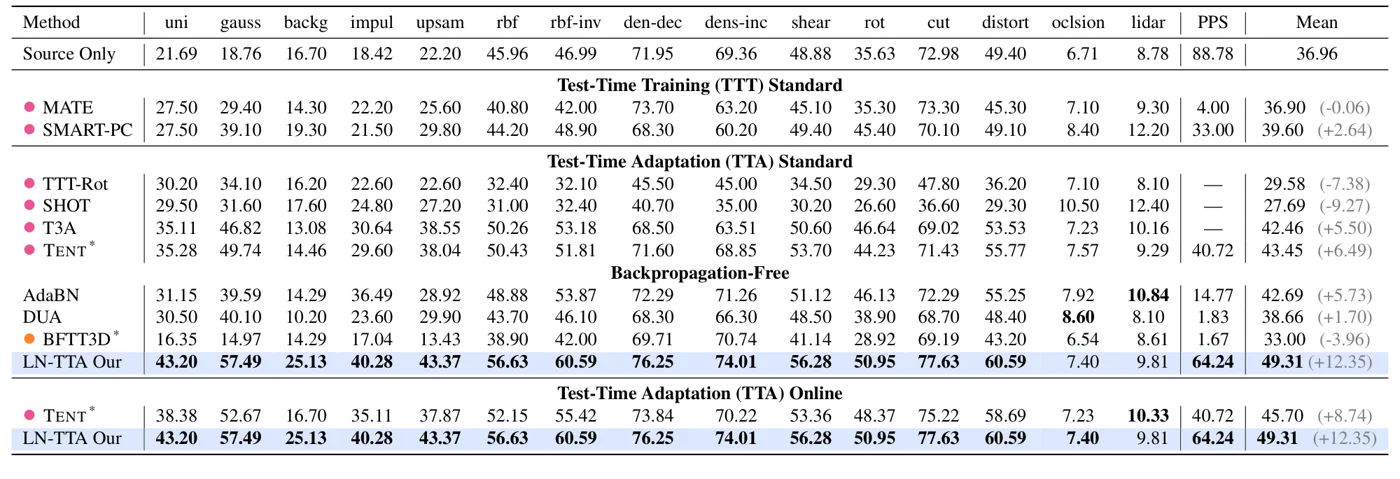 Table 1 of the paper: top-1 accuracy (%) for every ScanObjectNN-C corruption, with TTT, TTA, backprop-free, and online groups. Since LN-TTA keeps no state, its standard and online rows are the same. Figure from the paper.
LN-TTA has the best mean on ScanObjectNN-C and ModelNet40-C, with gains over Source Only of +12.35 and +15.58 points, and it beats backprop-based TENT in both standard and online modes. On ShapeNet-C the gain is only +3.03, and SMART-PC, a TTT method that changes pretraining, is 0.02 points higher (64.40 vs 64.38); LN-TTA is best among the backprop-free methods there. It runs at a large fraction of Source Only speed, and peak GPU memory at batch size 32 is 1.468 GB versus 2.890 GB for TENT and 7.443 GB for BFTT3D.
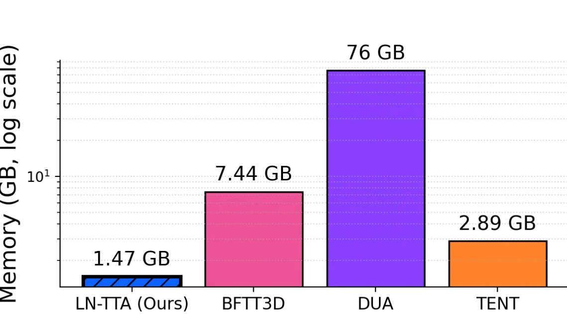 Total GPU memory (backbone plus data) at \(B = 32\), on a log scale. LN-TTA stores no backward graph, optimizer state, or feature bank, so it stays near Source Only, while DUA reaches 76 GB. Figure from the paper.
The paper also checks the theory empirically. It sweeps batch size \(B\) and feature dimension \(d\), and measures the Jensen-Shannon distance between the averaged per-feature post-LN batch marginal and \(\mathcal{N}(0,1)\).
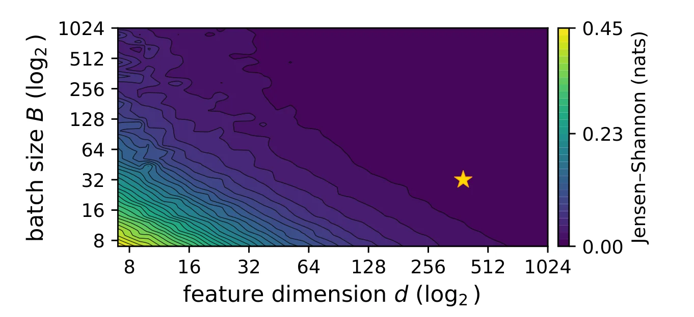 The distance shrinks as either \(B\) or \(d\) grows, and faster along \(d\). The star marks the setting used in the TTA experiments, which is already in the near-zero region. Figure from the paper.
Limitations
- The authors state that performance still depends on batch size, and that extending to other modalities and backbones is future work. The supplement shows accuracy rising with batch size on ShapeNet-C.
- All experiments use a single backbone (Point-MAE). The method needs LN layers and a [cls] token, so it does not apply to BN-only point networks such as PointNet or DGCNN.
- The recolouring in Eq. 16 uses only the prototype and the source LN parameters. It is the same fixed reparameterization for every target domain and does not read any statistics from the test batch.
- The supplement says the setup follows TENT in resetting BN statistics. AdaBN alone already reaches 67.91 on ModelNet40-C. The paper has no ablation that separates the BN reset from the LN edit, so it is unclear how much of the gain comes from each part.
- The theory is asymptotic (\(d, B \to \infty\), \(\varepsilon = 0\), i.i.d. samples). Using the [cls]-only forward pass as a proxy for source moments is motivated, not proven.
- Occlusion and LiDAR stay very low (7.40 and 9.81 on ScanObjectNN-C), and on ShapeNet-C DUA does better on these two.