Abstract
Point cloud TTA methods mostly adapt the model with several backpropagation steps. That makes them slow and sensitive to the number of update steps. Some, like MATE, also need an auxiliary task at training time, so they cannot be applied to an arbitrary pre-trained model. BFTT3D avoids backpropagation, but it needs class-level source prototypes at test time and is heavy in time and memory.
Purge-Gate (PG) works at the token level. Corruptions such as background points or impulse noise hit some local patches much harder than others. PG measures how far each token is from a source prototype and removes the most divergent tokens before the attention layers. Nothing is updated. There are two variants: PG-SP uses stored source statistics, and PG-SF is fully source-free and uses the model’s own [cls] token as the prototype.
Motivation
The paper starts from a difference between images and point clouds. In 2D TTA, the input has a fixed size and a corruption is usually spread evenly over the image. In a point cloud, a shift can add new points (background clutter, impulse outliers) or perturb only some regions of the shape. So the damage is uneven: a few local patches are badly corrupted while the rest of the object is almost clean. Existing point cloud TTA methods ignore this and adapt the whole model, either with backpropagation (TENT, MATE, SMART-PC) or with class-level source prototypes (BFTT3D).
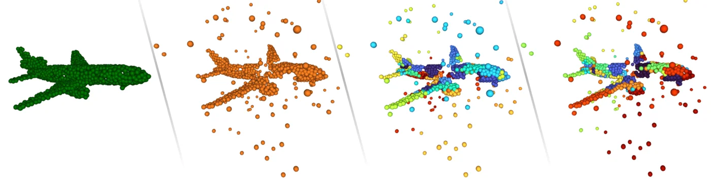 From left to right: a clean airplane, the same shape corrupted with stray outlier points, its tokens ranked by PG-SF, and its tokens ranked by PG-SP. Red marks the most shifted tokens. Both scores put the stray outlier patches at the top, while patches on the fuselage and wings stay low. Figure from the paper.
The figure is the core observation: the shift is concentrated in specific tokens, and a simple distance to a source prototype is enough to find them. The analysis in the Method section explains why those tokens matter. Once noise dominates a token, its LayerNorm output points in a near-random direction, and the attention layer drifts toward uniform weights. The key insight is borrowed from token pruning in efficient transformers (e.g. Kim et al., 2022), which drops uninformative tokens to save compute. Purge-Gate drops the most shifted tokens instead, to protect attention from them. This needs no gradient step and no change to the weights.
Method
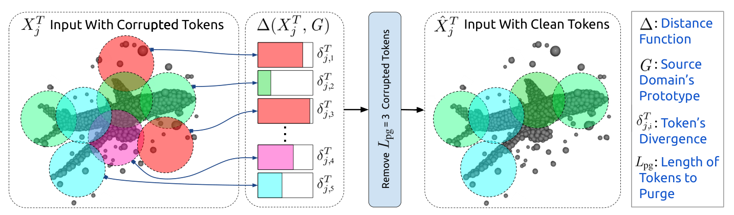 The input tokens \(X_j^T\) are scored by a distance \(\Delta\) to the source prototype \(G\). The \(L_{\text{pg}}\) most divergent tokens are removed, giving the purified input \(\hat{X}_j^T\). Figure from the paper.
Tokens
The backbone is a Point-MAE style transformer. A point cloud is split into \(L_t\) tokens. Each token \(x_{i,t} = (c_t, \mathcal{N}_t)\) is a center \(c_t\) chosen by farthest point sampling plus its \(k\) nearest neighbours \(\mathcal{N}_t\). These are the colored patches on the left of the figure.
Why noisy tokens hurt attention
The paper models the shift as additive noise on the embeddings, \(x_{j,t}^T = x_{j,t}^S + \epsilon_{j,t}\). LayerNorm is locally Lipschitz, so small noise keeps a token close to its clean version. When the noise dominates, \(\mathit{LN}(x_{j,t}^T) \approx \mathit{LN}(\epsilon_{j,t})\), which is close to a random direction in high dimension. Random directions are nearly orthogonal, so the attention scores to such tokens go to about zero, and the softmax drifts toward uniform weights:
\[A_{ij} = \frac{\exp(S_{ij}/\sqrt{d})}{\sum_k \exp(S_{ik}/\sqrt{d})} \approx \frac{1}{L_t}\]Uniform attention means the layer stops aggregating useful information. So the idea is to remove the noise-dominated tokens before they enter attention.
The gate
This is the middle of the figure. PG computes a distance between every target token and a source prototype \(G\):
\[\Delta(X_j^T, G) = (\delta_{j,1}^T, \delta_{j,2}^T, \dots, \delta_{j,L_t}^T)\]Then it drops the \(L_{\text{pg}}\) tokens with the largest distance:
\[\hat{X}_j^T = X_j^T \setminus \big\{ x_{j,t}^T \mid t \in \arg\max_{S \subseteq [L_t],\, |S| = L_{\text{pg}}} \sum_{t \in S} \delta_{j,t}^T \big\}\]The purge size is fixed per forward pass so that the batch can still be processed in parallel. The only open question is how to choose \(G\) and \(\Delta\).
PG-SP: source prototype
\(G = (\mu_S, \sigma_S)\) is the mean and standard deviation of source token embeddings. They are collected either (a) by one pass over the source data with Welford’s online algorithm, or (b) by a modified first LayerNorm that accumulates these statistics during training. The distance is a diagonal Mahalanobis distance:
\[\Delta(X_j^T, G) = \sqrt{(X_j^T - \mu_S)^T \Sigma_S^{-1} (X_j^T - \mu_S)}, \qquad \Sigma_S = \text{diag}(\sigma_S^2)\]PG-SF: source-free prototype
The learnable [cls] token is trained to attend to and summarize the source tokens. So PG-SF uses it, projected to query space, as a one-vector prototype, \(G = \mathit{LN}([\texttt{cls}])W_Q\). Each token’s key is compared with it by negative cosine similarity:
\[\Delta(X_j^T, G) = -\frac{(\mathit{LN}(X_j^T)W_K)\, G}{\|\mathit{LN}(X_j^T)W_K\| \cdot \|G\|}\]Tokens that the [cls] query would barely attend to are the ones purged.
Choosing the purge size, and BatchNorm
The best purge size depends on the corruption, and it cannot be learned without gradients. PG runs the model for a small set \(\mathcal{L}_{\text{pg}} = \{0, 2, 4, 8, 16, 32\}\) and keeps the output with the lowest entropy:
\[L_{\text{pg}}^* = \arg\min_{L \in \mathcal{L}_{\text{pg}}} H(f(x; L))\]Finally, since there is no adaptation pass, BatchNorm layers are reset to use the current batch statistics in each forward pass.
Main Experiments
Mean top-1 accuracy (%, higher is better) over 15 corruptions. All methods use the Point-MAE backbone released by MATE. Batch size 32, one iteration, model reset after each batch. This is the “Mean” column of Tables 1 to 3; the paper also lists per-corruption accuracies. Rows marked * were reproduced by the authors. MATE and SMART-PC need a training-time auxiliary task, and their numbers come from the SMART-PC paper.
| Method | Type | ScanObjectNN-C | ModelNet40-C | ShapeNet-C |
|---|---|---|---|---|
| Source Only | – | 36.96 | 54.16 | 61.35 |
| MATE | TTT | 36.90 | 58.90 | 63.10 |
| SMART-PC | TTT | 39.60 | 63.10 | 64.40 |
| TTT-Rot | TTA, backprop | 29.58 | 53.05 | 60.93 |
| SHOT | TTA, backprop | 27.69 | 26.60 | 36.19 |
| T3A* | TTA, backprop | 42.46 | 57.22 | 54.18 |
| TENT* | TTA, backprop | 43.45 | 63.53 | 54.98 |
| DUA | TTA, BP-free | 38.66 | 54.73 | 60.77 |
| BFTT3D* | TTA, BP-free | 33.00 | 57.16 | 60.73 |
| PG-SP | TTA, BP-free | 49.13 | 68.93 | 64.17 |
| PG-SF | TTA, BP-free, source-free | 47.54 | 68.68 | 64.40 |
For ShapeNet-C, the MATE and SMART-PC rows are the “Standard” variants.
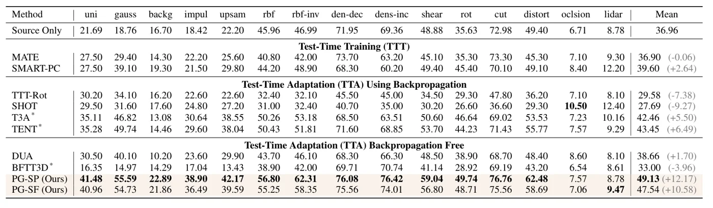 Table 1 of the paper: top-1 accuracy on each of the 15 ScanObjectNN-C corruptions, with the change over Source Only in parentheses. PG-SP is best on 13 of 15 corruptions. The two exceptions are occlusion and LiDAR, where every method stays at about 12% or below. Figure from the paper.
The per-corruption view shows where purging helps most. The biggest gains are on noise that adds or moves points: uniform noise (21.69 to 41.48), Gaussian noise (18.76 to 55.59) and impulse noise (18.42 to 38.90). Occlusion and LiDAR remove parts of the shape instead of adding bad points, so there is little to purge, and PG-SP gains almost nothing there.
Cost against BFTT3D (batch size 32, one NVIDIA A6000; the six purge sizes were run one after another, not in parallel):
| Method | Time per batch | GPU memory |
|---|---|---|
| BFTT3D | 173.94 ms | 7400 MiB |
| PG-SP | 14.07 ms | 1300 MiB |
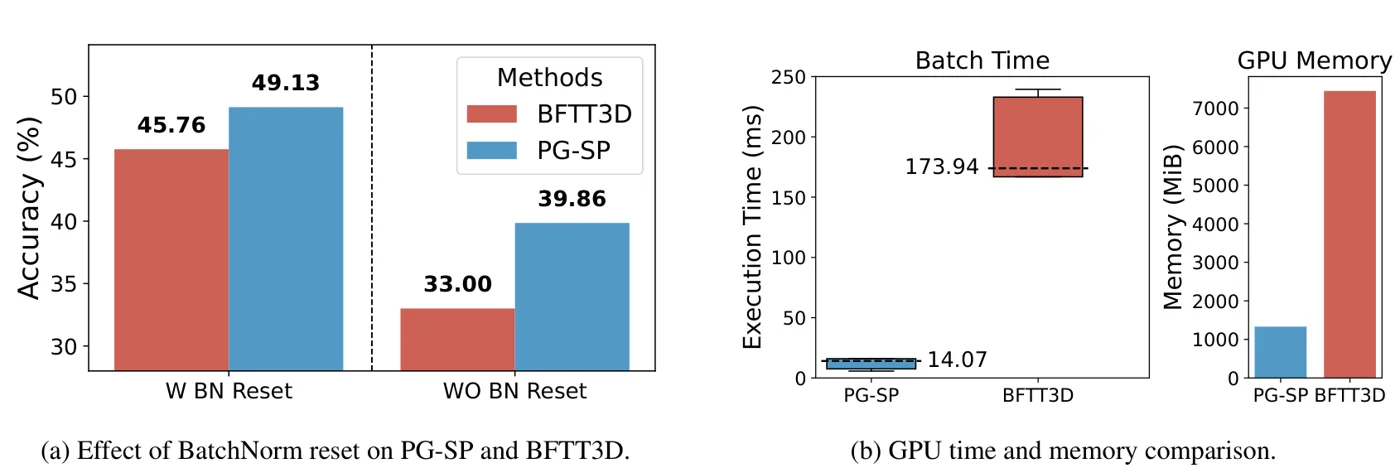 (a) Mean accuracy on ScanObjectNN-C with and without the BatchNorm reset, for PG-SP and BFTT3D. (b) Time per batch and GPU memory at batch size 32. PG-SP stays ahead in both settings of (a), but the reset alone moves BFTT3D from 33.00 to 45.76. Figure from the paper.
Panel (a) separates the two ingredients. Without the reset, PG-SP still beats BFTT3D by about 7 points (39.86 vs. 33.00), which is the effect of purging alone. With the reset on both, the gap shrinks to about 3 points. Panel (b) is the cost table above as a plot.
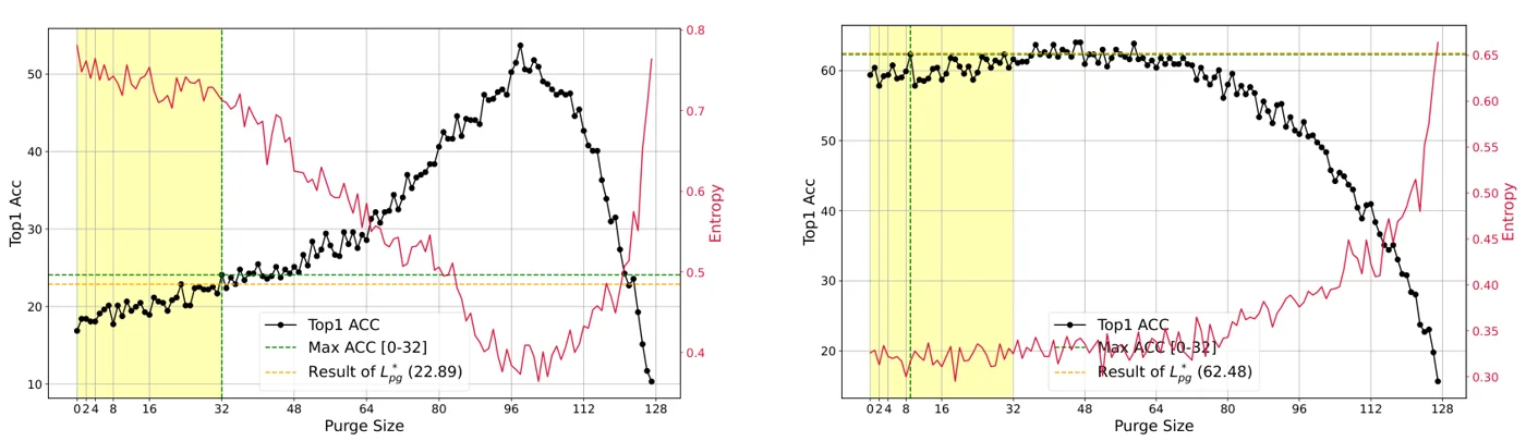 Accuracy (black) and output entropy (red) for every purge size from 0 to 127, on Background (left) and Distortion (right) corruption from ScanObjectNN-C. The yellow band is the searched range [0, 32]. The orange line is the accuracy reached by the entropy-based choice among the six sizes, and the green line is the best accuracy inside [0, 32]. Figure from the paper.
This plot shows why entropy is a reasonable selector. As the purge size grows, accuracy rises while entropy falls, and past about 100 tokens both turn: accuracy collapses and entropy jumps. Within [0, 32], the entropy choice lands close to the best value (22.89 vs. about 24 on Background, 62.48 on Distortion). But on Background, the true peak is above 50% at around 100 purged tokens, far outside the search range.
PG-SP and PG-SF give the best mean accuracy on ScanObjectNN-C and ModelNet40-C, ahead of TENT and the TTT methods, without any gradient step. ShapeNet-C is harder: most TTA methods fall below Source Only, and PG gains about 3 points, tied with SMART-PC. PG-SP is 12.4 times faster than BFTT3D and uses 5.5 times less memory. With a Point-Mamba backbone (Table 4), PG-SP improves ScanObjectNN-C from 29.11 to 41.42 and ModelNet-C from 58.32 to 68.61, but is slightly below Source Only on ShapeNet-C (51.66 vs. 51.92).
Limitations
The paper has no limitations section. Grounded observations:
- Several forward passes per batch. The purge-size search runs the model once per value in \(\mathcal{L}_{\text{pg}}\) (six values). This runs in parallel or sequentially, so it costs either more memory or more time than a single pass.
- The search window can be too small. The supplementary shows that heavy corruption needs far more purging. For background corruption at severity 7, accuracy peaks near \(L_{\text{pg}} \approx 112\) (33%), while the best value in \([0, 32]\) gives only 16%. The fixed set \(\{0, 2, 4, 8, 16, 32\}\) cannot reach that.
- BatchNorm reset matters a lot. PG-SP drops from 49.13 to 39.86 on ScanObjectNN-C without it. The same reset lifts BFTT3D from 33.00 to 45.76, while Table 1 lists BFTT3D at 33.00. Part of the headline gap over BFTT3D is the reset, not the purging. The reset also depends on batch statistics. The batch-size study (ShapeNet-C) shows accuracy still rises with batch size, though PG-SP stays above TENT at every size.
- Source access or retraining for PG-SP. PG-SP needs either source data for the statistics or a model trained with a modified LayerNorm. PG-SF avoids this but needs a [cls] token and query/key projections, so it is tied to transformer classifiers. The Mamba experiments use PG-SP only.
- Global token distance only. A token far from the source mean is not always corrupted. Purging too much removes informative tokens, and accuracy drops sharply past about 80 to 100 purged tokens in the ablations.
- Synthetic shifts dominate. Real-world shifts are tested only on two ScanObjectNN variants, with smaller gains (+1.38 on OBJ-BG, +4.30 on PB-T50-RS).