Abstract
Zero-shot CLIP is fairly well calibrated. The usual ways to adapt it, few-shot adapters (CLIP-Adapter, TIP-Adapter, TaskRes), prompt learning (CoOp, CoCoOp, MaPLe), and test-time prompt tuning (TPT), raise accuracy but make confidence worse, and the gap is largest on out-of-distribution data such as the ImageNet shifts. Standard fixes do not fit this setting: temperature scaling needs a labeled validation set from the test distribution, and a recent explanation for miscalibration in supervised training (logit norm growth, addressed by LogitNorm) does not match what happens here.
The paper argues that the cause is the growth of the logit range (max minus min logit), not the logit norm. It then constrains each sample’s logits to stay within the range of its own zero-shot logits. Three versions are given: ZS-Norm and Penalty act during adaptation, and SaLS (Sample-adaptive Logit Scaling) is a post-hoc rescaling at inference that works on any adapted model, including TPT.
Motivation
The starting observation is that adaptation buys accuracy at the cost of calibration, and that this holds for every family of CLIP adaptation, not only for one method. The authors show it with reliability diagrams on two ImageNet shifts. Zero-shot CLIP sits close to the diagonal (ECE 2.87 on ImageNet-V2, 3.14 on Sketch). After CoOp, CLIP-Adapter, or TPT, the bars fall below the diagonal, which means the model is more confident than it is accurate, and ECE rises to 9.40 (CLIP-Adapter) and 13.77 (TPT) on V2 and up to 15.28 (TPT) on Sketch.
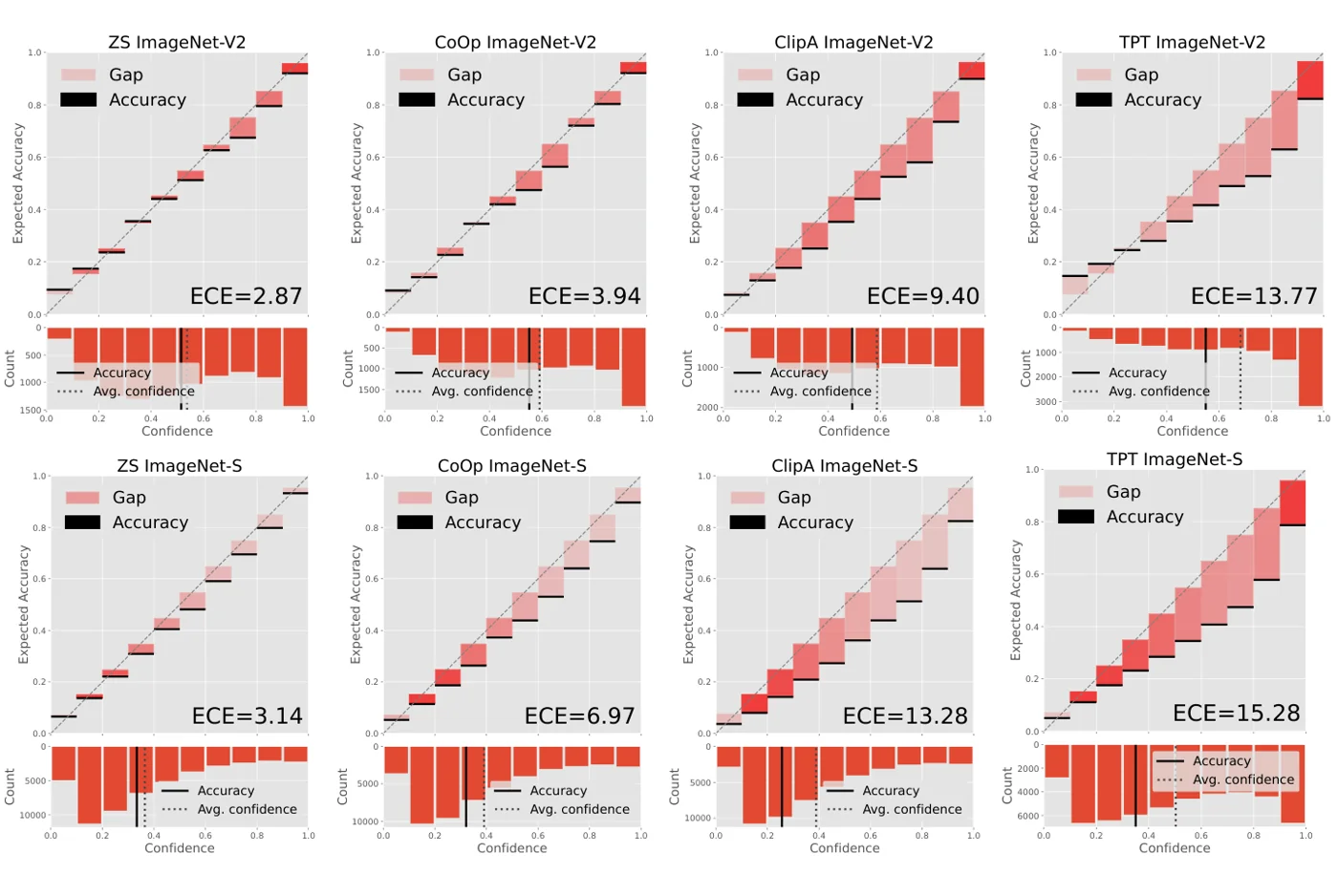 Reliability diagrams on ImageNet-V2 (top) and ImageNet-Sketch (bottom) for zero-shot CLIP, CoOp, CLIP-Adapter, and TPT. Every adaptation family pushes the bars below the diagonal (overconfidence); TPT is the worst. Figure from the paper.
Two gaps in prior work make this hard to fix. Temperature scaling and similar post-hoc methods need labeled data from the test distribution, which is not available under shift or at test time. And the explanation that comes from supervised training, that overconfidence follows from a growing logit norm, does not match CLIP adaptation: as the norm-vs-range plot in the Method section shows, the norm often drops after adaptation while ECE rises. What does move together with ECE is the logit range. That gives the key insight the method builds on: zero-shot CLIP already provides a well-calibrated, label-free reference range for every sample, so the adapted logits can simply be held to it.
Method
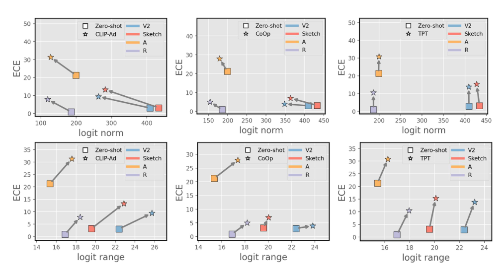 ECE against logit norm (top) and logit range (bottom) on ImageNet-V2/Sketch/A/R, for zero-shot CLIP (squares) and the adapted model (stars): CLIP-Adapter, CoOp, and TPT. After adaptation the norm often goes down while ECE goes up, but the range goes up together with ECE. The paper has no pipeline figure; this motivating figure is its core argument. Figure from the paper.
Norm or range?
Write the logit vector as \(\boldsymbol{l} = \lVert\boldsymbol{l}\rVert\,\hat{\boldsymbol{l}}\). Prior work on supervised networks blamed the growth of \(\lVert\boldsymbol{l}\rVert\) for overconfidence. Two simple facts separate norm from range:
- Adding a constant \(a>0\) to all non-negative logits increases the norm but leaves the softmax unchanged (Proposition 1). So a larger norm does not by itself mean higher confidence.
- With range \(R(\boldsymbol{l})=\max(\boldsymbol{l})-\min(\boldsymbol{l})\), scaling by \(a>1\) increases both the range and the top-class probability (Proposition 2).
The figure above checks this empirically. In all three families, the move from zero-shot (square) to adapted (star) increases ECE and logit range together, while the logit norm often decreases. The same reasoning covers TPT, since minimizing entropy pushes the winning logit away from the others.
The constraint
The goal is to train with the usual objective \(\mathcal{H}\) (cross-entropy for few-shot methods, entropy for TPT) while keeping every logit inside the zero-shot min and max of the same sample:
\[\min\ \mathcal{H}(\boldsymbol{Y},\boldsymbol{P}) \quad \text{s.t.} \quad l^{\text{ZS-min}}_{i}\mathbf{1}\leq\boldsymbol{l}_{i}\leq l^{\text{ZS-max}}_{i}\mathbf{1}\quad\forall i.\]Lagrangian methods are hard to use with deep models, so the paper gives three approximations.
ZS-Norm and Penalty (during adaptation)
ZS-Norm rescales the logits before the loss with a min-max map onto the zero-shot range:
\[\boldsymbol{l}^{\prime}_{i}=\frac{l^{\text{ZS-max}}_{i}-l^{\text{ZS-min}}_{i}}{l^{\text{max}}_{i}-l^{\text{min}}_{i}}\left(\boldsymbol{l}_{i}-l^{\text{min}}_{i}\mathbf{1}\right)+l^{\text{ZS-min}}_{i}\mathbf{1}.\]Penalty keeps the raw logits and adds a ReLU penalty for every logit outside the zero-shot range, with \(\lambda=10\):
\[\mathcal{H}(\boldsymbol{Y},\boldsymbol{P})+\lambda\sum_{i}\sum_{k=1}^{K}\left(\text{ReLU}(l_{ik}-l^{\text{ZS-max}}_{i})+\text{ReLU}(l^{\text{ZS-min}}_{i}-l_{ik})\right).\]SaLS (at inference)
SaLS applies the same min-max map \(\boldsymbol{l}^{\prime}_{i}\) only at test time, to the logits of an already adapted model. For each test sample it runs the zero-shot model once to get \(l^{\text{ZS-min}}_{i}\) and \(l^{\text{ZS-max}}_{i}\), rescales the adapted logits into that interval, and takes the softmax. The map is a positive affine transform per sample, so the predicted class does not change and accuracy is exactly that of the base method. The authors describe it as an unsupervised, per-sample temperature scaling: the temperature is set by the ratio of zero-shot range to adapted range, with no validation data.
Shrinking the range further is not better. Scaling the zero-shot range down to 1/2 or 1/4 in SaLS increases ECE again, since predictions become close to uniform.
Main Experiments
Test-time prompt tuning, 11 fine-grained datasets (average). Accuracy and ECE in %. RN50 numbers are from the main paper (Table 3), ViT-B/16 from the appendix (Table 9). SaLS leaves accuracy unchanged by construction.
| Method | RN50 Acc | RN50 ECE | ViT-B/16 Acc | ViT-B/16 ECE |
|---|---|---|---|---|
| Zero-shot | 56.03 | 5.04 | 63.92 | 3.91 |
| TPT | 58.03 | 11.27 | 65.18 | 11.36 |
| TPT w/ ZS-Norm | 57.94 | 10.57 | 65.13 | 10.82 |
| TPT w/ Penalty | 57.69 | 9.58 | 65.22 | 9.27 |
| TPT w/ SaLS | 58.03 | 9.26 | 65.18 | 9.88 |
| C-TPT | 57.54 | 6.33 | 64.59 | 4.81 |
| C-TPT w/ ZS-Norm | 57.63 | 5.74 | 64.41 | 5.03 |
| C-TPT w/ Penalty | 57.52 | 3.14 | 64.68 | 4.61 |
| C-TPT w/ SaLS | 57.54 | 5.22 | 64.59 | 4.48 |
Note: in the paper’s RN50 table, the C-TPT average ECE values do not match the mean of the listed per-dataset values (for C-TPT w/ Penalty, the per-dataset values average 5.93, which is the number printed in the ImageNet column; the TPT rows do match). The numbers above are copied as printed.
The per-dataset version of this table (RN50) shows where the TPT gains come from. SaLS helps most on the datasets where TPT is worst calibrated, such as EuroSAT (21.00 to 12.31) and DTD (25.29 to 21.09), and changes little where TPT is already close to zero-shot (Caltech, Pets).
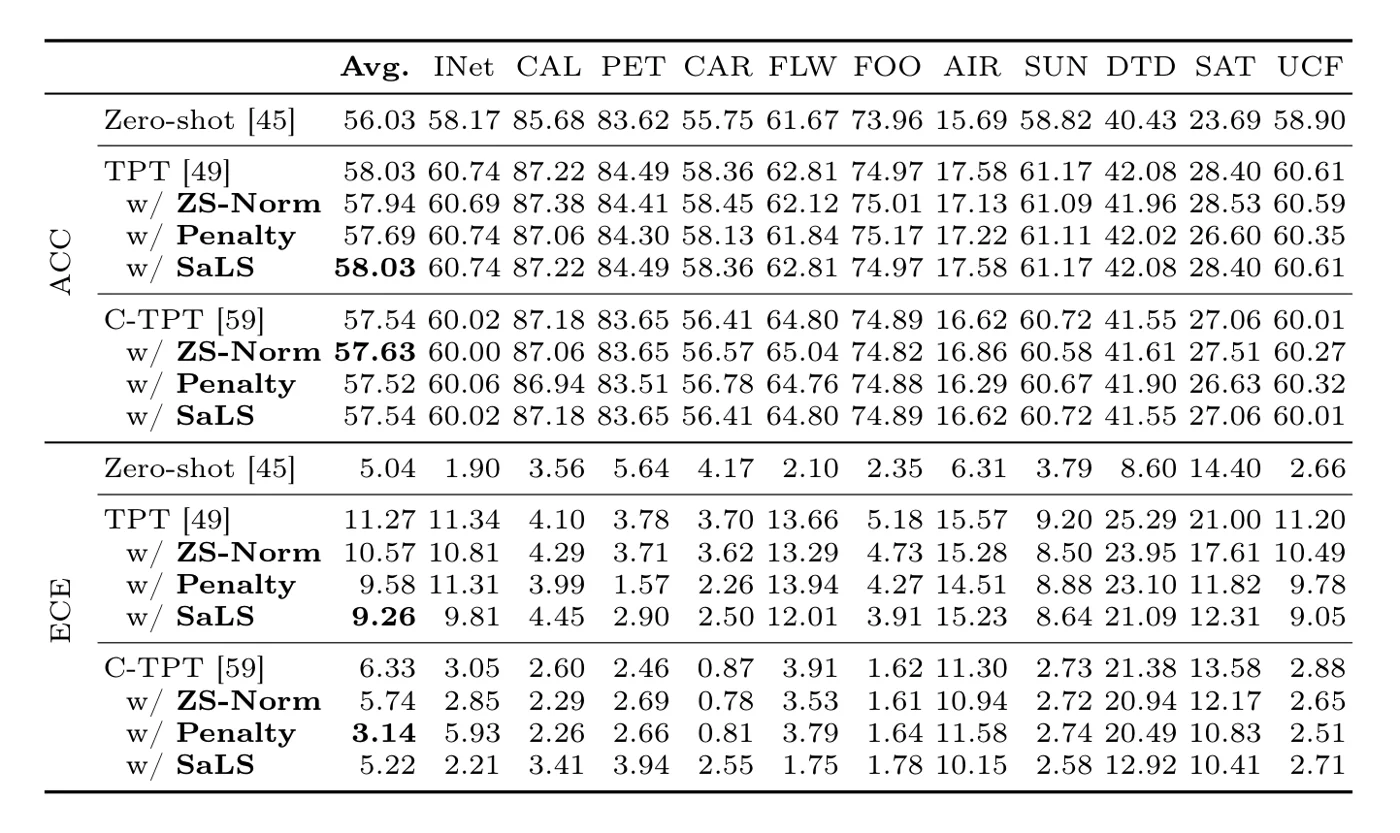 Table 3 of the paper: accuracy (top) and ECE (bottom) on ImageNet and 10 fine-grained datasets with RN50, for TPT and C-TPT with ZS-Norm, Penalty, and SaLS. The accuracy rows for SaLS are identical to their base method. Figure from the paper.
The reliability diagrams for TPT with ViT-B/16 make the same point visually. On StanfordCars the differences are small, while on EuroSAT TPT is badly overconfident (ECE 20.42) and SaLS pulls the bars back toward the diagonal (13.88), though Penalty does better (8.53).
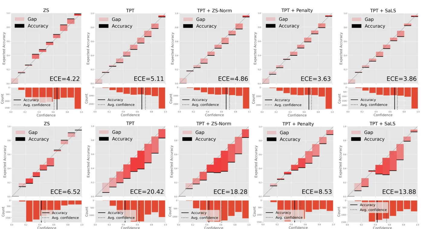 Reliability diagrams on StanfordCars (top) and EuroSAT (bottom) for zero-shot, TPT, TPT + ZS-Norm, TPT + Penalty, and TPT + SaLS (ViT-B/16). On EuroSAT the gap between confidence and accuracy shrinks a lot with Penalty and less with SaLS. Figure from the paper.
Few-shot adaptation (16-shot ImageNet), ViT-B/16, average over ImageNet-V2/Sketch/A/R. From Tables 1(b) and 2(d). Zero-shot is 57.15 / 4.78. Each cell is Acc / ECE.
| Method | Base | w/ Penalty | w/ SaLS |
|---|---|---|---|
| CLIP-Adapter | 50.61 / 7.82 | 51.59 / 6.38 | 50.61 / 4.38 |
| TIP-Adapter(f) | 25.86 / 63.63 | 49.23 / 40.98 | 25.86 / 44.37 |
| TaskRes | 58.01 / 7.52 | 58.31 / 6.65 | 58.01 / 6.21 |
| CoOp | 58.41 / 6.61 | 59.18 / 4.91 | 58.41 / 4.90 |
| CoCoOp | 59.74 / 4.83 | 60.20 / 3.89 | 59.74 / 4.81 |
| MaPLe | 60.07 / 4.13 | 60.62 / 3.78 | 60.07 / 4.38 |
For TPT, SaLS lowers ECE by about 1.5 to 2 points on fine-grained data with no accuracy change, but the result (9.26 and 9.88) stays far above zero-shot and above C-TPT. On top of C-TPT it gives the lowest ViT-B/16 ECE in the table (4.48). On the ImageNet shifts with TPT (appendix Table 8), the effect is smaller: 17.58 to 16.74 ECE with RN50 and 11.81 to 10.86 with ViT-B/16. In few-shot adaptation the gains are larger for adapters (for example CLIP-Adapter 7.82 to 4.38), while for strong prompt learners like CoCoOp and MaPLe it changes little or slightly worsens ECE, and Penalty is often as good or better.
The authors also check that the fix acts on the quantity they blamed. After calibration with SaLS, the mean logit range goes down on all four ImageNet shifts for CLIP-Adapter, CoOp, and TPT, while the logit norm goes up for CLIP-Adapter and CoOp. This is consistent with the claim that range, not norm, is what matters.
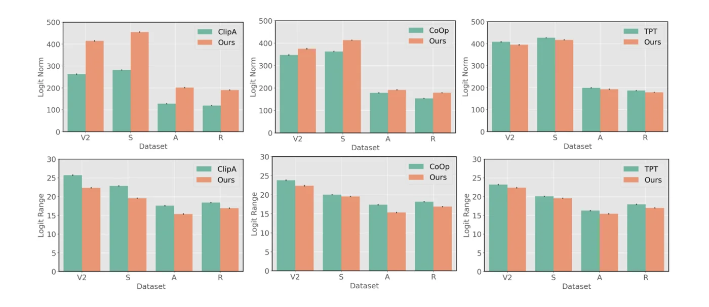 Mean logit norm (top) and logit range (bottom) on ImageNet-V2/Sketch/A/R for CLIP-Adapter, CoOp, and TPT, without and with SaLS (“Ours”). Calibration lowers the range everywhere, while the norm often increases. Figure from the paper.
Limitations
- Assumes zero-shot is a good reference. The target range comes from zero-shot CLIP. Where zero-shot is itself poorly calibrated (ImageNet-A has 21.32 ECE with RN50 zero-shot), matching its range cannot fix much.
- Modest effect on TPT alone. TPT w/ SaLS still has roughly twice the zero-shot ECE on fine-grained datasets and much higher ECE on the ImageNet shifts. Later work (CoTS) reports SaLS as the weakest of the TPT calibration baselines it compares.
- Not uniformly helpful. SaLS increases ECE for MaPLe (4.13 to 4.38) and leaves CoCoOp almost unchanged; ZS-Norm hurts CLIP-Adapter accuracy and ECE. The best variant depends on the method.
- Only the range is controlled. The rescaling sets the gap between the max and min logit, but not how the other logits are spread inside that interval.
- Extra zero-shot pass. Each test sample needs zero-shot logits in addition to the adapted ones. For TPT the zero-shot logits are already computed, and CoTS measures no added time for SaLS, but for other adapted models it is a second forward pass.
- Reporting inconsistency. Some RN50 C-TPT averages in Table 3 do not match their per-dataset values, which makes the C-TPT comparison on RN50 hard to read.