- 파이토치 한번에 끝내기 (이수안컴퓨터연구소) 1편 정리
- Colab 노트북
- 코드: 노트북의 각 실습 설명에 맞춰 작성
노트북의 코드 셀은 비어 있는 실습용 템플릿이다. 이 글의 코드는 각 셀 앞의 설명에 맞춰 PyTorch 2.x(CPU)에서 직접 작성하고 실행한 것이며, 출력도 그 실행 결과다. 무작위 값이 들어가는 셀은 실행할 때마다 숫자가 달라진다.
파이토치(PyTorch)
PyTorch는 페이스북(현 Meta)이 루아(Lua) 언어로 개발되었던 토치(Torch)를 파이썬 버전으로 다시 만들어 2017년에 공개한 라이브러리다. 초기의 Torch는 NumPy처럼 과학 연산을 위한 라이브러리였으며, 이후 GPU를 이용한 텐서 조작과 동적 신경망 구축이 가능한 딥러닝 프레임워크로 발전했다. 파이썬다운(pythonic) 문법으로 작성할 수 있어 유연하면서도, GPU 가속으로 빠른 계산 속도를 제공한다는 점이 특징이다.
파이토치 모듈 구조
PyTorch는 세 층으로 이루어져 있다. 가장 위의 Top-level API는 torch, torch.autograd, torch.nn 등 사용자가 직접 쓰는 파이썬 패키지이고, 가운데의 Mid-level Engine은 Autograd, ATen, JIT 같은 C++ 엔진이며, 가장 아래의 Low-level Library는 CPU(TH, THNN)와 CUDA(THC, THCUNN)용 C/CUDA 구현이다. 아래층의 구현은 자동으로 감싸져(auto wrapping) 위층의 파이썬 API로 노출된다. 노트북은 이 구조를 Manning의 Deep Learning with PyTorch(Eli Stevens, Luca Antiga) 그림으로 소개한다.
파이토치의 구성요소
| 패키지 | 역할 |
|---|---|
torch |
메인 네임스페이스. 텐서와 다양한 수학 함수를 포함한다. |
torch.autograd |
자동 미분 기능을 제공한다. |
torch.nn |
신경망 구축을 위한 데이터 구조와 레이어를 제공한다. |
torch.multiprocessing |
병렬 처리 기능을 제공한다. |
torch.optim |
SGD(Stochastic Gradient Descent)를 중심으로 한 파라미터 최적화 알고리즘을 제공한다. |
torch.utils |
데이터 조작 등 유틸리티 기능을 제공한다. |
torch.onnx |
ONNX(Open Neural Network Exchange) 형식으로 내보내 서로 다른 프레임워크 사이에서 모델을 공유할 때 쓴다. |
텐서(Tensors)
PyTorch는 데이터를 표현하는 기본 구조로 텐서(tensor)를 사용한다. 텐서는 데이터를 담는 컨테이너로, 일반적으로 수치형 데이터를 저장한다. NumPy의 ndarray와 비슷하지만 GPU를 사용해 연산을 가속할 수 있다는 차이가 있다.
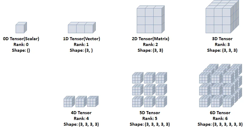 0차원(스칼라)부터 6차원까지의 텐서. 차원 수(rank)가 하나 늘 때마다 아래 차원의 텐서를 여러 개 늘어놓은 모양이 되며, 모양(shape)에도 숫자가 하나씩 추가된다. 출처: 이수안컴퓨터연구소 Colab 노트북.
먼저 PyTorch를 불러오고 버전을 확인한다.
import torch
print(torch.__version__)
2.14.1+cpu
텐서 초기화와 데이터 타입
초기화되지 않은 텐서는 torch.empty()로 만든다. 메모리를 할당만 하고 값을 채우지 않으므로, 그 자리에 원래 있던 값이 그대로 보인다.
x = torch.empty(4, 2)
print(x)
tensor([[0., 0.],
        [0., 0.],
        [0., 0.],
        [0., 0.]])
이번 실행에서는 모두 0이 나왔지만, 환경에 따라 아주 크거나 작은 임의의 값이 나올 수 있다. 값이 정해져 있지 않으므로 바로 계산에 쓰지 않는다.
무작위로 초기화된 텐서는 torch.rand()로 만든다. 값은 \([0, 1)\) 구간의 균등분포에서 뽑힌다.
torch.manual_seed(42)
x = torch.rand(4, 2)
print(x)
tensor([[0.8823, 0.9150],
        [0.3829, 0.9593],
        [0.3904, 0.6009],
        [0.2566, 0.7936]])
torch.manual_seed()로 시드를 고정했으므로 같은 값을 다시 얻을 수 있다.
데이터 타입(dtype)이 long이고 0으로 채워진 텐서는 torch.zeros()에 dtype=torch.long을 넘긴다.
x = torch.zeros(4, 2, dtype=torch.long)
print(x)
tensor([[0, 0],
        [0, 0],
        [0, 0],
        [0, 0]])
정수형이므로 0.이 아니라 0으로 출력된다. torch.long은 torch.int64와 같다.
사용자가 입력한 값으로 텐서를 초기화할 때는 torch.tensor()에 리스트를 넘긴다.
x = torch.tensor([3, 2.3])
print(x)
tensor([3.0000, 2.3000])
정수 3과 실수 2.3이 섞여 있으므로 둘 다 담을 수 있는 torch.float32로 정해진다.
2 x 4 크기, double 타입, 1로 채워진 텐서는 기존 텐서의 new_ones()로 만들 수 있다. new_* 메서드는 원래 텐서의 속성(장치 등)을 이어받되, 인자로 준 크기와 자료형을 적용한다.
x = x.new_ones(2, 4, dtype=torch.double)
print(x)
tensor([[1., 1., 1., 1.],
        [1., 1., 1., 1.]], dtype=torch.float64)
기본 자료형(float32)이 아닐 때만 출력에 dtype이 함께 표시된다.
x와 같은 크기, float 타입, 무작위로 채워진 텐서는 torch.randn_like()로 만든다. _like 함수는 입력 텐서와 같은 크기의 텐서를 만들며, dtype을 주면 자료형만 바꾼다. randn은 표준정규분포에서 값을 뽑는다.
x = torch.randn_like(x, dtype=torch.float)
print(x)
tensor([[-1.1229, -0.1863,  2.2082, -0.6380],
        [ 0.4617,  0.2674,  0.5349,  0.8094]])
텐서의 크기는 size() 또는 shape로 확인한다.
print(x.size())
print(x.shape)
print(x.numel())   # 전체 원소 수
torch.Size([2, 4])
torch.Size([2, 4])
8
torch.Size는 튜플의 하위 클래스이므로 rows, cols = x.size()처럼 풀어 쓸 수 있다.
데이터 타입(Data Type)
| Data type | dtype | CPU tensor | GPU tensor |
|---|---|---|---|
| 32-bit floating point | torch.float32 or torch.float |
torch.FloatTensor |
torch.cuda.FloatTensor |
| 64-bit floating point | torch.float64 or torch.double |
torch.DoubleTensor |
torch.cuda.DoubleTensor |
| 16-bit floating point | torch.float16 or torch.half |
torch.HalfTensor |
torch.cuda.HalfTensor |
| 8-bit integer (unsigned) | torch.uint8 |
torch.ByteTensor |
torch.cuda.ByteTensor |
| 8-bit integer (signed) | torch.int8 |
torch.CharTensor |
torch.cuda.CharTensor |
| 16-bit integer (signed) | torch.int16 or torch.short |
torch.ShortTensor |
torch.cuda.ShortTensor |
| 32-bit integer (signed) | torch.int32 or torch.int |
torch.IntTensor |
torch.cuda.IntTensor |
| 64-bit integer (signed) | torch.int64 or torch.long |
torch.LongTensor |
torch.cuda.LongTensor |
표의 torch.FloatTensor 같은 텐서 타입 클래스로 직접 텐서를 만들 수 있다. 다만 현재 PyTorch에서는 torch.tensor(..., dtype=torch.float32)처럼 dtype을 지정하는 방식이 권장된다.
ft = torch.FloatTensor([1, 2, 3])
print(ft)
print(ft.dtype)
tensor([1., 2., 3.])
torch.float32
텐서의 short(), int(), long() 메서드로 정수형으로 변환한다.
print(ft.short())
print(ft.int())
print(ft.long())
tensor([1, 2, 3], dtype=torch.int16)
tensor([1, 2, 3], dtype=torch.int32)
tensor([1, 2, 3])
정수형의 기본값은 int64이므로 long()의 결과에는 dtype이 표시되지 않는다.
it = torch.IntTensor([1, 2, 3])
print(it)
print(it.dtype)
tensor([1, 2, 3], dtype=torch.int32)
torch.int32
반대로 float(), double(), half()로 정수형을 부동소수점형으로 바꾼다.
print(it.float())
print(it.double())
print(it.half())
tensor([1., 2., 3.])
tensor([1., 2., 3.], dtype=torch.float64)
tensor([1., 2., 3.], dtype=torch.float16)
이 메서드들은 모두 to(dtype)의 축약형이며, 예를 들어 it.float()은 it.to(torch.float32)와 같다.
CUDA Tensors
.to() 메서드를 사용하면 텐서를 CPU나 GPU 등 어떤 장치로도 옮길 수 있다. 먼저 원소가 하나인 텐서를 만들고, item()으로 파이썬 숫자를 꺼내 본다.
x = torch.randn(1)
print(x)
print(x.item())
print(x.dtype)
tensor([1.1103])
1.110290288925171
torch.float32
GPU를 쓸 수 있으면 cuda, 아니면 cpu를 장치로 정하고, 텐서를 그 장치에서 만들거나 그 장치로 옮겨 연산한다.
device = torch.device("cuda" if torch.cuda.is_available() else "cpu")
print(device)
y = torch.ones_like(x, device=device)   # 처음부터 device에 생성
x = x.to(device)                        # device로 이동
z = x + y
print(z)
print(z.to("cpu", torch.double))        # 장치와 자료형을 함께 변경
cpu
tensor([2.1103])
tensor([2.1103], dtype=torch.float64)
이 출력은 GPU가 없는 환경의 결과다. GPU가 있는 Colab에서 실행하면 device가 cuda가 되고 z는 tensor([...], device='cuda:0')처럼 장치가 함께 표시된다. 연산에 쓰는 두 텐서는 반드시 같은 장치에 있어야 한다.
다차원 텐서 표현
0D Tensor(Scalar) 는 숫자 하나를 담은 텐서로, 축(axis)과 형상(shape)이 없다.
t0 = torch.tensor(0)
print(t0.ndim)
print(t0.shape)
print(t0)
0
torch.Size([])
tensor(0)
1D Tensor(Vector) 는 값들을 나열한 리스트와 비슷한 텐서로, 축이 하나 있다.
t1 = torch.tensor([1, 2, 3])
print(t1.ndim)
print(t1.shape)
print(t1)
1
torch.Size([3])
tensor([1, 2, 3])
2D Tensor(Matrix) 는 행렬과 같은 모양으로 축이 두 개다. 일반적인 수치, 통계 데이터셋이 여기에 해당하며, 주로 샘플(samples)과 특성(features)을 가진 구조로 쓴다.
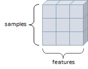 2D 텐서. 세로 축은 샘플, 가로 축은 특성이다. 출처: 이수안컴퓨터연구소 Colab 노트북.
t2 = torch.tensor([[1, 2, 3],
                   [4, 5, 6],
                   [7, 8, 9]])
print(t2.ndim)
print(t2.shape)
print(t2)
2
torch.Size([3, 3])
tensor([[1, 2, 3],
        [4, 5, 6],
        [7, 8, 9]])
3D Tensor 는 큐브(cube)와 같은 모양으로 축이 세 개다. 연속된 시퀀스 데이터나 시간 축이 포함된 시계열 데이터가 여기에 해당하며, 주식 가격 데이터셋이나 시간에 따른 질병 발병 데이터 등이 그 예다. 주로 샘플(samples), 타임스텝(timesteps), 특성(features)을 가진 구조로 쓴다.
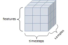 3D 텐서. 앞면의 세로 축은 특성, 가로 축은 타임스텝이고, 깊이 방향으로 샘플이 쌓인다. 출처: 이수안컴퓨터연구소 Colab 노트북.
t3 = torch.tensor([[[1, 2, 3], [4, 5, 6], [7, 8, 9]],
                   [[1, 2, 3], [4, 5, 6], [7, 8, 9]],
                   [[1, 2, 3], [4, 5, 6], [7, 8, 9]]])
print(t3.ndim)
print(t3.shape)
print(t3)
3
torch.Size([3, 3, 3])
tensor([[[1, 2, 3],
         [4, 5, 6],
         [7, 8, 9]],

        [[1, 2, 3],
         [4, 5, 6],
         [7, 8, 9]],

        [[1, 2, 3],
         [4, 5, 6],
         [7, 8, 9]]])
3×3 행렬이 3개 쌓인 모양이며, 출력에서 빈 줄이 가장 바깥 축(첫 번째 축)의 경계를 나타낸다.
4D Tensor 는 축이 4개다. 컬러 이미지 데이터가 대표적인 예이며(흑백 이미지는 채널이 하나라 3D 텐서로도 표현할 수 있다), 주로 샘플(samples), 높이(height), 너비(width), 컬러 채널(channel)을 가진 구조로 쓴다.
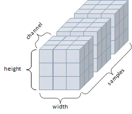 4D 텐서. 높이, 너비, 채널로 이루어진 이미지 한 장이 큐브 하나이고, 이런 큐브가 샘플 축을 따라 여러 개 놓인다. 출처: 이수안컴퓨터연구소 Colab 노트북.
그림은 채널을 마지막 축으로 두는 표현이지만, PyTorch의 이미지 텐서는 관례적으로 (N, C, H, W), 즉 채널을 높이와 너비 앞에 둔다.
5D Tensor 는 축이 5개다. 비디오 데이터가 대표적인 예이며, 주로 샘플(samples), 프레임(frames), 높이(height), 너비(width), 컬러 채널(channel)을 가진 구조로 쓴다.
텐서의 연산(Operations)
텐서에 대해 수학 연산, 삼각함수, 비트 연산, 비교 연산, 집계 등 다양한 연산이 제공된다. 먼저 원소별 수학 연산이다.
a = torch.tensor([[-0.7, 0.3]])
print(a)
print(torch.abs(a))               # 절댓값
print(torch.ceil(a))              # 올림
print(torch.floor(a))             # 내림
print(torch.clamp(a, -0.5, 0.5))  # [-0.5, 0.5] 범위로 자르기
tensor([[-0.7000,  0.3000]])
tensor([[0.7000, 0.3000]])
tensor([[-0., 1.]])
tensor([[-1.,  0.]])
tensor([[-0.5000,  0.3000]])
ceil(-0.7)은 -0.으로 표시되는데, 부동소수점의 음의 0이며 값은 0과 같다. clamp는 범위를 벗어난 값만 경계값으로 바꾼다.
다음은 텐서 전체를 하나의 값으로 줄이는 집계 연산이다.
print(a)
print(torch.min(a))
print(torch.max(a))
print(torch.mean(a))
print(torch.std(a))    # 표준편차
print(torch.prod(a))   # 모든 원소의 곱
print(torch.unique(torch.tensor([1, 2, 3, 1, 2, 2])))  # 중복 제거
tensor([[-0.7000,  0.3000]])
tensor(-0.7000)
tensor(0.3000)
tensor(-0.2000)
tensor(0.7071)
tensor(-0.2100)
tensor([1, 2, 3])
torch.std()는 기본적으로 표본 표준편차(n-1로 나눔)를 계산하므로 두 값 -0.7, 0.3의 표준편차가 \(\sqrt{0.5} \approx 0.7071\)이 된다.
max와 min은 dim 인자를 주면 최댓값(최솟값)과 함께 그 위치도 반환한다. argmax는 최댓값을 가진 인덱스, argmin은 최솟값을 가진 인덱스다.
x = torch.tensor([[0.2, 0.8, 0.4],
                  [0.5, 0.1, 0.9]])
print(x)
print(x.max(dim=0))
print(x.max(dim=1))
tensor([[0.2000, 0.8000, 0.4000],
        [0.5000, 0.1000, 0.9000]])
torch.return_types.max(
values=tensor([0.5000, 0.8000, 0.9000]),
indices=tensor([1, 0, 1]))
torch.return_types.max(
values=tensor([0.8000, 0.9000]),
indices=tensor([1, 2]))
dim=0은 행 방향(위아래)으로 비교해 열마다 하나씩, dim=1은 열 방향(좌우)으로 비교해 행마다 하나씩 결과를 낸다. 지정한 차원이 사라진다고 생각하면 결과 모양을 쉽게 알 수 있다.
print(x.min(dim=0))
print(x.min(dim=1))
torch.return_types.min(
values=tensor([0.2000, 0.1000, 0.4000]),
indices=tensor([0, 1, 0]))
torch.return_types.min(
values=tensor([0.2000, 0.1000]),
indices=tensor([0, 1]))
반환값은 이름 있는 튜플이므로 값과 인덱스를 나눠 받을 수 있고, 인덱스만 필요하면 argmax()를 쓴다.
values, indices = x.max(dim=1)
print(values)
print(indices)
print(x.argmax(dim=1))
tensor([0.8000, 0.9000])
tensor([1, 2])
tensor([1, 2])
torch.add는 덧셈이다. 연산자 +, 함수 torch.add(), 메서드 x.add()가 모두 같은 결과를 낸다.
x = torch.tensor([[1., 2.], [3., 4.]])
y = torch.tensor([[5., 6.], [7., 8.]])
print(x + y)
print(torch.add(x, y))
print(x.add(y))
tensor([[ 6.,  8.],
        [10., 12.]])
tensor([[ 6.,  8.],
        [10., 12.]])
tensor([[ 6.,  8.],
        [10., 12.]])
결과를 담을 텐서를 out 인자로 제공할 수도 있다.
result = torch.empty(2, 2)
torch.add(x, y, out=result)
print(result)
tensor([[ 6.,  8.],
        [10., 12.]])
in-place 방식은 새 텐서를 만들지 않고 텐서 자체의 값을 바꾼다. 이런 연산은 이름 뒤에 밑줄 _이 붙으며, x.copy_(y), x.t_() 등이 그 예다.
print(y)
y.add_(x)   # y = y + x 를 y 자리에서 수행
print(y)
tensor([[5., 6.],
        [7., 8.]])
tensor([[ 6.,  8.],
        [10., 12.]])
y.add(x)는 y를 그대로 두고 새 텐서를 반환하지만, y.add_(x)는 y의 값을 직접 바꾼다.
torch.sub는 뺄셈이다.
y = torch.tensor([[5., 6.], [7., 8.]])
print(x - y)
print(torch.sub(x, y))
print(x.sub(y))
tensor([[-4., -4.],
        [-4., -4.]])
tensor([[-4., -4.],
        [-4., -4.]])
tensor([[-4., -4.],
        [-4., -4.]])
torch.mul은 곱셈이다. 같은 위치의 원소끼리 곱하는 원소별 곱셈이다.
print(x * y)
print(torch.mul(x, y))
print(x.mul(y))
tensor([[ 5., 12.],
        [21., 32.]])
tensor([[ 5., 12.],
        [21., 32.]])
tensor([[ 5., 12.],
        [21., 32.]])
torch.div는 나눗셈이다.
print(x / y)
print(torch.div(x, y))
print(x.div(y))
tensor([[0.2000, 0.3333],
        [0.4286, 0.5000]])
tensor([[0.2000, 0.3333],
        [0.4286, 0.5000]])
tensor([[0.2000, 0.3333],
        [0.4286, 0.5000]])
torch.mm은 행렬 곱이다. 노트북은 이를 내적(dot product)으로 소개하는데, 결과의 각 원소가 왼쪽 행렬의 행과 오른쪽 행렬의 열의 내적이기 때문이다. 1차원 벡터 두 개의 내적은 torch.dot()으로 계산한다.
print(torch.mm(x, y))
print(x @ y)
print(torch.dot(torch.tensor([1., 2.]), torch.tensor([3., 4.])))
tensor([[19., 22.],
        [43., 50.]])
tensor([[19., 22.],
        [43., 50.]])
tensor(11.)
예를 들어 결과의 왼쪽 위 19는 \(1 \cdot 5 + 2 \cdot 7\)이다. torch.mm()은 2차원 행렬 전용이고, 배치 차원까지 처리하려면 torch.matmul()이나 @를 쓴다.
텐서의 조작(Manipulations)
인덱싱(Indexing) 은 NumPy처럼 대괄호 인덱스로 사용할 수 있다.
x = torch.tensor([[1, 2],
                  [3, 4]])
print(x)
print(x[0, 0])
print(x[0, 1])
print(x[1, 0])
print(x[1, 1])
print(x[:, 0])   # 0번 열
print(x[:, 1])   # 1번 열
print(x[0, :])   # 0번 행
print(x[1, :])   # 1번 행
tensor([[1, 2],
        [3, 4]])
tensor(1)
tensor(2)
tensor(3)
tensor(4)
tensor([1, 3])
tensor([2, 4])
tensor([1, 2])
tensor([3, 4])
원소 하나를 골라도 결과는 0차원 텐서다. :는 그 축의 모든 값을 뜻한다.
view 는 텐서의 크기(size)나 모양(shape)을 바꾼다. 바꾸기 전과 후의 전체 원소 개수가 같아야 하며, 한 축을 -1로 두면 나머지 축과 원소 수로부터 그 크기를 계산해 채운다.
x = torch.randn(4, 5)
y = x.view(20)
z = x.view(5, -1)
print(x.size())
print(y.size())
print(z.size())
torch.Size([4, 5])
torch.Size([20])
torch.Size([5, 4])
원소가 20개이므로 view(5, -1)의 -1은 4로 정해진다. view는 데이터를 복사하지 않고 같은 메모리를 다른 모양으로 보여 주므로, y나 z를 수정하면 x도 바뀐다.
item 은 텐서에 값이 하나만 있을 때 그 값을 파이썬 숫자로 꺼낸다.
x = torch.tensor([2.5])
print(x)
print(x.item())
print(x.dtype)
tensor([2.5000])
2.5
torch.float32
값이 하나만 있어야 item()을 쓸 수 있으며, 원소가 둘 이상이면 오류가 난다.
x = torch.randn(2)
print(x)
print(x.item())
tensor([-1.6898,  0.1331])
RuntimeError: a Tensor with 2 elements cannot be converted to Scalar
여러 값을 파이썬 객체로 꺼내려면 tolist()를 쓴다.
squeeze 는 크기가 1인 차원을 축소(제거)한다.
tensor = torch.arange(1., 10.).reshape(1, 3, 3)
print(tensor)
print(tensor.shape)
tensor([[[1., 2., 3.],
         [4., 5., 6.],
         [7., 8., 9.]]])
torch.Size([1, 3, 3])
t = tensor.squeeze()
print(t)
print(t.shape)
tensor([[1., 2., 3.],
        [4., 5., 6.],
        [7., 8., 9.]])
torch.Size([3, 3])
맨 앞의 크기 1인 차원이 사라져 [1, 3, 3]이 [3, 3]이 되었다. squeeze(dim=0)처럼 차원을 지정하면 그 차원만 (크기가 1일 때) 제거한다.
unsqueeze 는 지정한 위치에 크기 1인 차원을 증가(생성)시킨다.
t = torch.arange(1., 10.).reshape(3, 3)
print(t.shape)
torch.Size([3, 3])
t1 = t.unsqueeze(dim=0)
print(t1)
print(t1.shape)
tensor([[[1., 2., 3.],
         [4., 5., 6.],
         [7., 8., 9.]]])
torch.Size([1, 3, 3])
t2 = t.unsqueeze(dim=2)
print(t2)
print(t2.shape)
tensor([[[1.],
         [2.],
         [3.]],

        [[4.],
         [5.],
         [6.]],

        [[7.],
         [8.],
         [9.]]])
torch.Size([3, 3, 1])
dim=0이면 맨 앞에, dim=2면 맨 뒤에 크기 1인 축이 생긴다. 이미지 한 장에 배치 차원을 붙이는 image.unsqueeze(0)이 대표적인 쓰임이다.
stack 은 같은 크기의 텐서들을 새 차원을 따라 쌓아 결합한다.
x = torch.tensor([1, 4])
y = torch.tensor([2, 5])
z = torch.tensor([3, 6])
print(torch.stack([x, y, z]))
print(torch.stack([x, y, z], dim=1))
tensor([[1, 4],
        [2, 5],
        [3, 6]])
tensor([[1, 2, 3],
        [4, 5, 6]])
길이 2인 벡터 세 개를 dim=0으로 쌓으면 (3, 2), dim=1로 쌓으면 (2, 3)이 된다.
cat 은 텐서를 이어 붙이는(concatenate) 메서드다. stack과 달리 새 차원을 만들지 않고, 이미 존재하는 차원을 따라 붙인다. 그래서 붙일 dim이 두 텐서에 이미 있어야 하고, 그 차원을 제외한 나머지 크기는 같아야 하며, 결과에서는 해당 차원의 크기가 늘어난다.
a = torch.ones(1, 3, 3)
b = torch.zeros(1, 3, 3)
c = torch.cat((a, b), dim=0)
print(c)
print(c.size())
tensor([[[1., 1., 1.],
         [1., 1., 1.],
         [1., 1., 1.]],

        [[0., 0., 0.],
         [0., 0., 0.],
         [0., 0., 0.]]])
torch.Size([2, 3, 3])
c = torch.cat((a, b), dim=1)
print(c)
print(c.size())
tensor([[[1., 1., 1.],
         [1., 1., 1.],
         [1., 1., 1.],
         [0., 0., 0.],
         [0., 0., 0.],
         [0., 0., 0.]]])
torch.Size([1, 6, 3])
c = torch.cat((a, b), dim=2)
print(c)
print(c.size())
tensor([[[1., 1., 1., 0., 0., 0.],
         [1., 1., 1., 0., 0., 0.],
         [1., 1., 1., 0., 0., 0.]]])
torch.Size([1, 3, 6])
1로 채운 a와 0으로 채운 b를 붙였으므로 어느 쪽 원소가 어디로 갔는지 바로 보인다. 지정한 차원의 크기만 3에서 6(dim=0에서는 1에서 2)으로 늘어났다.
chunk 는 텐서를 여러 조각으로 나눈다. “몇 개로 나눌 것인가”를 인자로 준다.
tensor = torch.arange(18).reshape(3, 6)
print(tensor)
t1, t2, t3 = torch.chunk(tensor, 3, dim=1)
print(t1)
print(t2)
print(t3)
tensor([[ 0,  1,  2,  3,  4,  5],
        [ 6,  7,  8,  9, 10, 11],
        [12, 13, 14, 15, 16, 17]])
tensor([[ 0,  1],
        [ 6,  7],
        [12, 13]])
tensor([[ 2,  3],
        [ 8,  9],
        [14, 15]])
tensor([[ 4,  5],
        [10, 11],
        [16, 17]])
열 6개를 3조각으로 나누었으므로 조각마다 열이 2개씩 들어갔다.
split 은 chunk와 같은 일을 하지만, “조각 하나의 크기가 몇인가”를 인자로 준다는 점이 다르다.
t1, t2 = torch.split(tensor, 3, dim=1)
print(t1)
print(t2)
print([p.shape for p in torch.split(tensor, [1, 2, 3], dim=1)])
tensor([[ 0,  1,  2],
        [ 6,  7,  8],
        [12, 13, 14]])
tensor([[ 3,  4,  5],
        [ 9, 10, 11],
        [15, 16, 17]])
[torch.Size([3, 1]), torch.Size([3, 2]), torch.Size([3, 3])]
같은 숫자 3이 chunk에서는 조각 수, split에서는 조각 크기를 뜻한다. split에는 리스트를 넘겨 조각마다 크기를 다르게 정할 수도 있다.
torch ↔ numpy: PyTorch 텐서는 numpy()로 NumPy 배열로, NumPy 배열은 torch.from_numpy()로 텐서로 변환할 수 있다. 텐서가 CPU에 있으면 두 객체가 메모리 공간을 공유하므로, 하나를 바꾸면 다른 하나도 바뀐다.
a = torch.ones(7)
print(a)
tensor([1., 1., 1., 1., 1., 1., 1.])
b = a.numpy()
print(b)
[1. 1. 1. 1. 1. 1. 1.]
a.add_(1)
print(a)
print(b)
tensor([2., 2., 2., 2., 2., 2., 2.])
[2. 2. 2. 2. 2. 2. 2.]
텐서 a만 in-place로 바꿨는데 배열 b도 2가 되었다. 메모리를 공유하기 때문이다.
import numpy as np
a = np.ones(7)
b = torch.from_numpy(a)
np.add(a, 1, out=a)
print(a)
print(b)
[2. 2. 2. 2. 2. 2. 2.]
tensor([2., 2., 2., 2., 2., 2., 2.], dtype=torch.float64)
반대 방향도 마찬가지다. NumPy의 기본 자료형이 float64이므로 변환된 텐서도 torch.float64다. 공유를 원하지 않으면 torch.tensor(a)로 복사본을 만든다.
정리
- PyTorch는 파이썬 API(Top-level) 아래에 C++ 엔진과 C/CUDA 라이브러리가 있는 구조이며,
torch,torch.autograd,torch.nn,torch.optim,torch.utils등의 패키지로 구성된다. - 텐서는
torch.empty,torch.rand,torch.zeros,torch.tensor,new_ones,randn_like등으로 만들고, 크기는size()나shape로 확인한다. - 자료형은
dtype으로 지정하며,float(),double(),int(),long()등으로 변환한다. 장치는to(device)로 옮긴다. - 0D(스칼라), 1D(벡터), 2D(행렬, 샘플×특성), 3D(시계열), 4D(이미지), 5D(비디오) 텐서가 데이터 종류에 대응한다.
- 원소별 연산(
add,sub,mul,div), 집계(min,max,mean,std), 행렬 곱(mm)을 제공하며, 이름 끝의_는 in-place 연산을 뜻한다. view,squeeze,unsqueeze로 모양을 바꾸고,stack(새 차원)과cat(기존 차원)으로 결합하며,chunk(조각 수)와split(조각 크기)으로 나눈다.- CPU 텐서와 NumPy 배열은
numpy(),from_numpy()로 변환하며 메모리를 공유한다.