Abstract
Large vision-language models (LVLMs) suffer from object hallucination: they describe objects that are not in the image. The paper points to two causes that earlier work had already identified: statistical bias from the training data (objects that are frequent or that co-occur with what is actually present) and language priors of the LLM decoder (what text usually says about a subject). Earlier fixes need extra cost, such as hallucination-targeted fine-tuning data, a trained post-hoc revisor, or factually augmented RLHF.
VCD needs no training and no external model. It runs the LVLM twice per token, once with the original image and once with a Gaussian-noised copy, and subtracts the second set of logits from the first. Because the noised image makes the model fall back on priors and biases, the subtraction removes exactly those tokens that the image does not support. An adaptive plausibility constraint keeps the subtraction from promoting nonsense tokens.
Motivation
The key claim is that visual uncertainty amplifies the two causes of hallucination. The authors blur the image with the forward diffusion process (Gaussian noise over \(T\) steps) and watch how the next-token distribution changes.
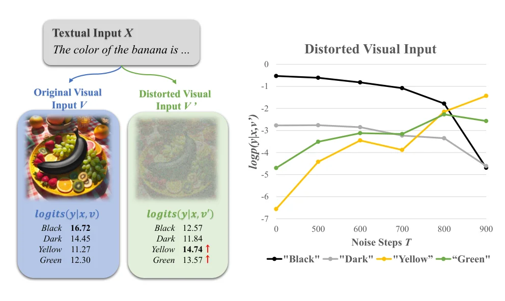 An image of a black banana with the prompt “The color of the banana is …”. With the original image, “Black” has the highest logit (16.72). With the distorted image, “Yellow” (14.74) and “Green” (13.57) take over. The right plot shows \(\log p(y \mid x, v')\) as noise steps grow: “Black” collapses while the conventional colors rise. Figure from the paper.
Language priors are one side. Statistical bias is the other: most vision-language pretraining data come from MSCOCO, with an unbalanced object distribution and biased co-occurrences. With distorted inputs, LLaVA-1.5 hallucinates frequent objects (person, dining table, car) and objects that co-occur with “dining table” (person, cup, bottle) more often than with the original image.
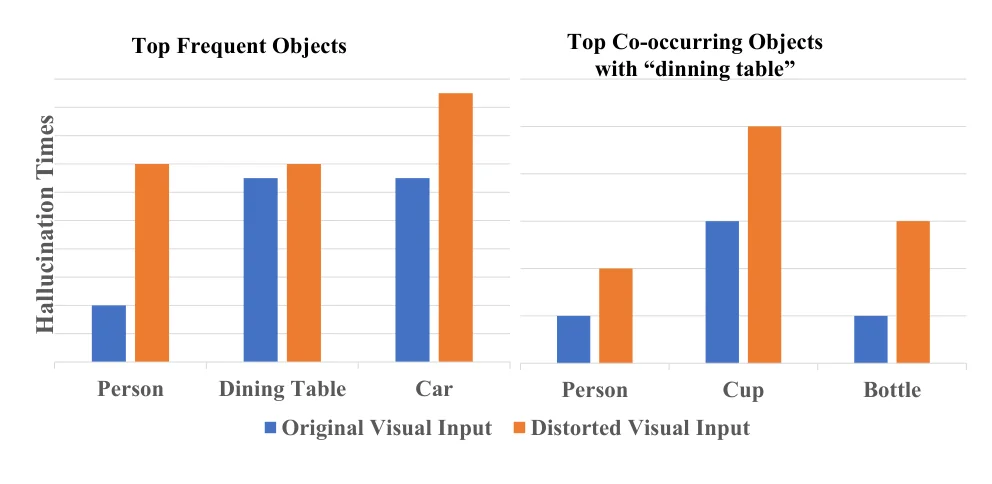 Left: the most frequent MSCOCO objects are hallucinated more often when the visual input is distorted. Right: the same holds for objects that often appear with “dining table”. Figure from the paper.
Directly on POPE, regular decoding with LLaVA-1.5 degrades steadily as noise grows: accuracy and F1 both fall, and F1 falls faster once \(T\) passes 500. The noised input is therefore a reliable way to produce a distribution that is more hallucinatory than the original, and that is what VCD uses as the negative.
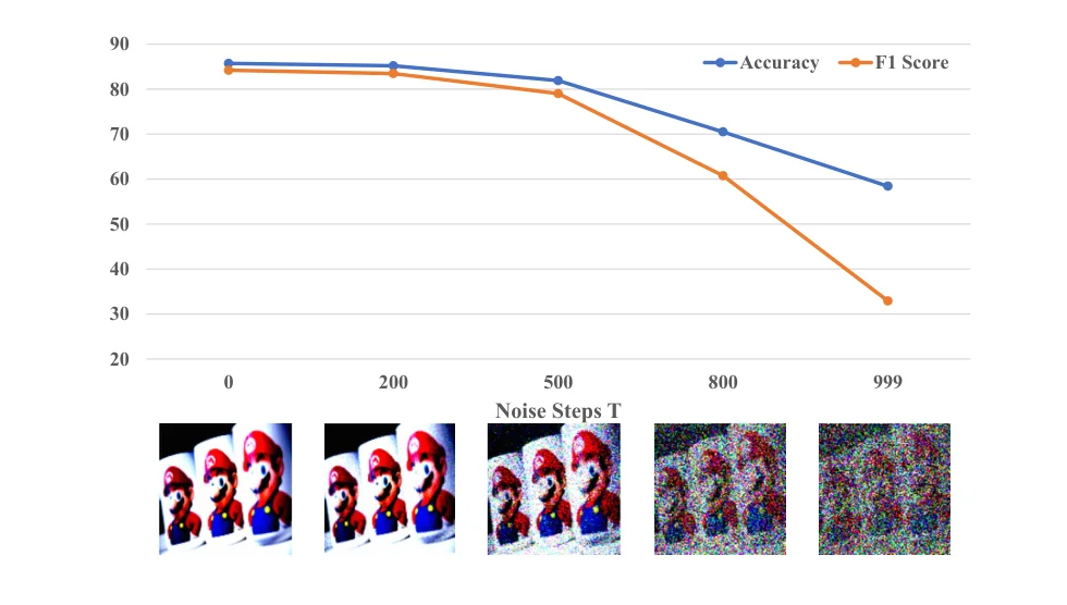 POPE accuracy and F1 of LLaVA-1.5 under regular decoding as the number of noise steps \(T\) grows, with the corresponding noised images below. Figure from the paper.
Method
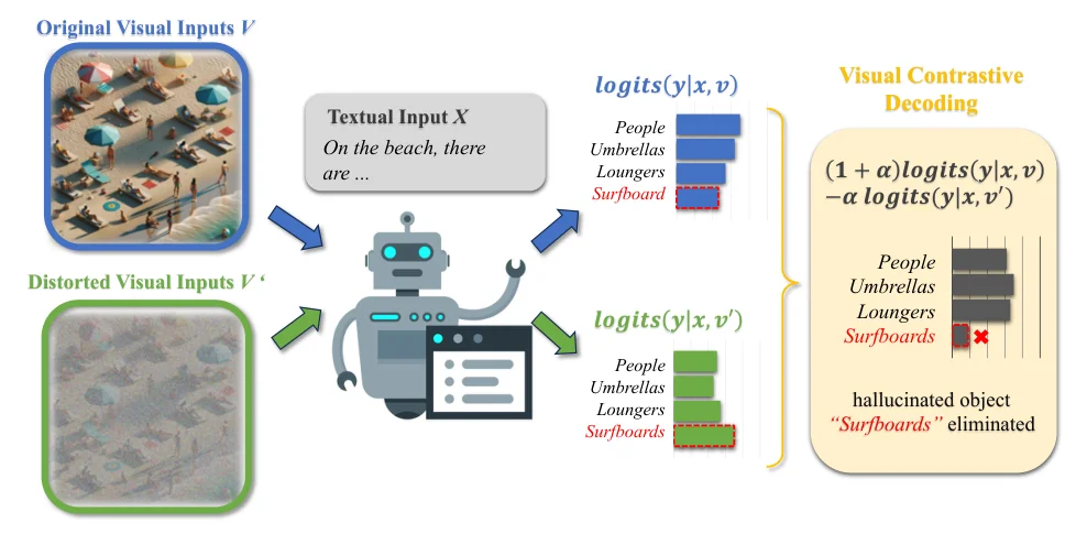 VCD on a beach image. The original image \(v\) and the distorted image \(v'\) both give logits for the next object. “Surfboards” is weak with \(v\) but strong with \(v'\), so the contrast removes it. Figure from the paper.
Visual uncertainty
The distorted image \(v'\) is produced with the forward diffusion process:
\[q(v_t \mid v_{t-1}) = \mathcal{N}\big(v_t;\ \sqrt{1-\gamma}\, v_{t-1},\ \gamma I\big), \qquad q(v_T \mid v_0) = \prod_{t=1}^{T} q(v_t \mid v_{t-1})\]with \(\gamma = 0.1\). \(T = 999\) is used for POPE and \(T = 500\) for MME and LLaVA-Bench.
Contrastive distribution
Given the query \(x\), VCD computes the logits with \(v\) and with \(v'\) and samples from
\[p_{\text{vcd}}(y \mid v, v', x) = \mathrm{softmax}\big[(1+\alpha)\,\mathrm{logit}_\theta(y \mid v, x) - \alpha\,\mathrm{logit}_\theta(y \mid v', x)\big]\]\(\alpha = 0\) is regular decoding, and the paper uses \(\alpha = 1\). The authors note the parallel to classifier-free guidance in diffusion models, \((1+\alpha)\epsilon_\theta(x, c) - \alpha \epsilon_\theta(x)\): here the “unconditional” branch is the model with a blurred image.
Adaptive plausibility constraint
Subtracting the whole distorted distribution is too aggressive, since the distorted branch still knows grammar and common sense. Following contrastive decoding for LLMs (Li et al.), VCD only keeps tokens that are already plausible under the original image:
\[\mathcal{V}_{\text{head}}(y_{<t}) = \big\{ y_t \in \mathcal{V} : p_\theta(y_t \mid v, x, y_{<t}) \ge \beta \max_w p_\theta(w \mid v, x, y_{<t}) \big\}\]and sets \(p_{\text{vcd}} = 0\) outside this set, with \(\beta = 0.1\). When the model is confident, the set often contains a single token, so VCD does not change easy decisions.
Main Experiments
All runs use direct sampling as the baseline (“Regular”) and report the mean over 5 runs. POPE on MSCOCO (accuracy / F1, Yes/No questions about object existence):
| Setting | Model | Regular Acc | VCD Acc | Regular F1 | VCD F1 |
|---|---|---|---|---|---|
| Random | LLaVA-1.5 | 83.29 | 87.73 | 81.33 | 87.16 |
| Random | Qwen-VL | 84.73 | 88.63 | 82.67 | 87.81 |
| Random | InstructBLIP | 80.71 | 84.53 | 80.41 | 83.68 |
| Popular | LLaVA-1.5 | 81.88 | 85.38 | 80.06 | 85.06 |
| Popular | Qwen-VL | 84.13 | 87.12 | 82.06 | 86.40 |
| Popular | InstructBLIP | 78.22 | 81.47 | 78.36 | 81.07 |
| Adversarial | LLaVA-1.5 | 78.96 | 80.88 | 77.57 | 81.33 |
| Adversarial | Qwen-VL | 82.26 | 84.26 | 80.37 | 83.90 |
| Adversarial | InstructBLIP | 75.84 | 79.56 | 76.59 | 79.52 |
MME hallucination subset (object-level: existence, count; attribute-level: position, color; score per subtask, max 200):
| Model | Decoding | Existence | Count | Position | Color | Total |
|---|---|---|---|---|---|---|
| LLaVA-1.5 | Regular | 175.67 | 124.67 | 114.00 | 151.00 | 565.33 |
| LLaVA-1.5 | VCD | 184.66 | 138.33 | 128.67 | 153.00 | 604.66 |
| Qwen-VL | Regular | 155.00 | 127.67 | 131.67 | 173.00 | 587.33 |
| Qwen-VL | VCD | 156.00 | 131.00 | 128.00 | 181.67 | 596.67 |
| InstructBLIP | Regular | 141.00 | 75.33 | 66.67 | 97.33 | 380.33 |
| InstructBLIP | VCD | 168.33 | 92.33 | 64.00 | 123.00 | 447.67 |
- VCD improves every POPE setting on every model, by up to +5.8 accuracy and +7.4 F1. On LLaVA-1.5 and Qwen-VL the F1 gain comes mostly from recall (up to about +10 points), while precision drops slightly. On InstructBLIP it comes from precision.
- On MME, object-level scores rise for all models. Position barely moves and even drops for Qwen-VL and InstructBLIP, which the authors read as LVLMs being weak at position reasoning in the first place.
- With GPT-4V as a judge on LLaVA-Bench (scale of 10), accuracy goes 3.23 → 4.15 (LLaVA-1.5), 3.84 → 4.23 (InstructBLIP) and 4.76 → 6.69 (Qwen-VL), and detailedness rises too.
On the full MME with LLaVA-1.5, VCD raises every perception subtask. Recognition stays about the same, with small drops on numerical calculation and text translation.
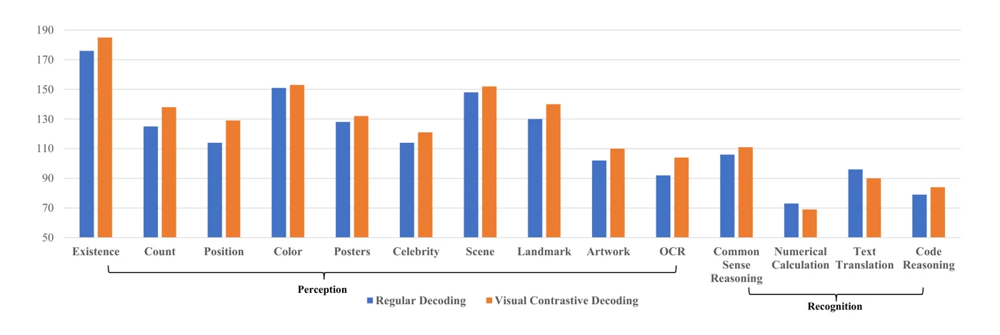 MME full set on LLaVA-1.5. VCD (orange) beats regular decoding (blue) on all ten perception subtasks. On the four recognition subtasks it is mixed. Figure from the paper.
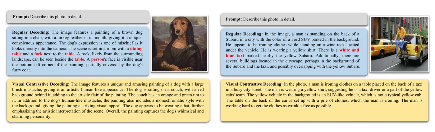 Two LLaVA-Bench cases. Regular decoding adds objects that co-occur with the scene (“dining table”, “fork”, “white and blue taxi”, in red). VCD describes the dog painting and the man ironing on a taxi without them. Figure from the paper.
Limitations
- Twice the forward cost. Every token needs a second pass with the distorted image.
- A crude distortion. The authors themselves say Gaussian noise is the most basic choice and that finer distortions, such as object-level blurring, might work better. They also limit the study to images, not video.
- A weak baseline. Regular decoding means direct sampling from the softmax. Gains over greedy or beam search are only shown in the supplement, on POPE-Random.
- Sensitive to \(\beta\). In the supplement, raising \(\beta\) from 0.1 to 0.5 lifts the MME hallucination subset of LLaVA-1.5 from 591.67 to 635.00, so the plausibility constraint does much of the work and the default setting is not tuned.
- Precision can drop. On POPE, LLaVA-1.5 and Qwen-VL lose precision under VCD (for example 83.06 → 79.45 on MSCOCO adversarial for LLaVA-1.5), so the model says “yes” more often. The F1 gain hides a shift in the yes/no balance.