Abstract
CLIP can classify images zero-shot by comparing an image with text such as “a photo of a dog”. The choice of prompt matters, and hand-crafted prompts need domain heuristics. Prompt tuning methods like CoOp and CoCoOp learn the prompt instead, but they need labeled training data from the downstream task, and the learned prompt tends to fit that task’s distribution. On datasets with larger shifts, the paper finds they show no advantage over an ensemble of hand-crafted prompts.
Test-time prompt tuning (TPT) learns the prompt from the single test sample it is about to classify. No training data and no labels are used. For image classification, TPT makes many augmented views of the test image, keeps the most confident ones, and updates the prompt so the averaged prediction over those views has low entropy. The same idea is also adapted to a context-dependent visual reasoning task (Bongard-HOI).
Motivation
Prompt tuning treats the prompt embeddings like model weights and fits them to labeled data from a downstream task. The authors argue that the learned prompt is then tied to that training distribution. Table 1 already hints at this: CoOp and CoCoOp, trained on ImageNet, gain most on ImageNet and ImageNet-V2, which are close to the training data, but on ImageNet-A, -R, and -Sketch they are no better than an ensemble of 80 hand-crafted prompts.
The cleaner evidence is a cross-dataset transfer test. A prompt is tuned on one fine-grained dataset (16 shots) and evaluated on another, and the accuracy is reported relative to zero-shot CLIP with a hand-crafted prompt, \((acc - acc_{\text{base}})/acc_{\text{base}}\). For example, CLIP-RN50 gets 61.75% on Flower102 with “a photo of a”, but CoOp trained on DTD gets only 33.41% there, a relative change of \(-0.46\).
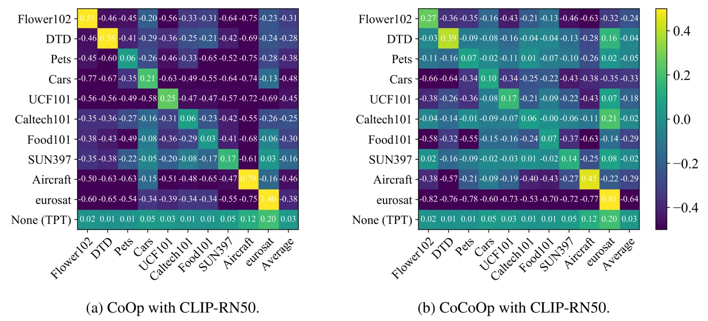 Relative accuracy change over zero-shot CLIP-RN50 when a prompt tuned on the row dataset is tested on the column dataset, for CoOp (a) and CoCoOp (b). Only the diagonal is positive; the bottom row (TPT, no source dataset) is positive everywhere. Figure from the paper.
Off the diagonal almost every cell is negative, so a prompt tuned on one dataset usually hurts on another, and the Average column is negative for every source dataset. CoCoOp’s image-conditioned prompt makes most cells less negative but does not remove the drop. This motivates the key idea: instead of learning one prompt from a training distribution, learn a prompt for each test sample from that sample alone. Since there is no label, the signal must be unsupervised, and the paper uses consistency of predictions across augmented views. The bottom row, TPT, improves on all 10 datasets.
Method
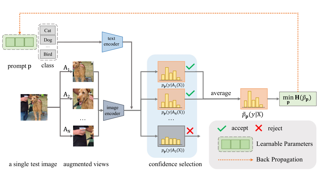 TPT for image classification. A single test image is augmented into N views, low-confidence views are rejected, and the prompt is updated to minimise the entropy of the averaged prediction. Figure from the paper.
CLIP with a prompt
CLIP has an image encoder and a text encoder. For a \(K\)-class problem, a prompt \(\mathbf{p}\) is prepended to each class name \(y_i\), and the text encoder gives one feature \(\mathbf{t}_i\) per class. The image feature \(\mathbf{v}\) is compared to each text feature with cosine similarity, and a softmax over the scaled similarities gives \(p(y_i \mid X)\). In zero-shot CLIP, \(\mathbf{p}\) is the fixed text “a photo of a”. In prompt tuning, \(\mathbf{p} \in \mathbb{R}^{L\times D}\) is a set of \(L\) learnable token embeddings in the text input space. Only the prompt is learned; both encoders stay frozen.
The authors choose the prompt as the parameter to adapt because it changes the input context without touching the pre-trained features. In an ablation with MEMO-style test-time optimisation (Figure 4a), tuning the prompt beats tuning the whole model, the text encoder, or the visual encoder. Tuning the visual encoder is the worst.
Marginal entropy over augmented views
There is no label at test time, so TPT needs an unsupervised objective. It generates \(N\) augmented views \(\mathcal{A}_i(X_{\text{test}})\) and averages the predicted class distributions:
\[\tilde{p}_{\mathbf{p}}(y \mid X_{\text{test}}) = \frac{1}{N}\sum_{i=1}^{N} p_{\mathbf{p}}(y \mid \mathcal{A}_i(X_{\text{test}})).\]The prompt is updated to minimise the entropy of this average:
\[\mathbf{p}^{*} = \arg\min_{\mathbf{p}} -\sum_{i=1}^{K} \tilde{p}_{\mathbf{p}}(y_i \mid X_{\text{test}}) \log \tilde{p}_{\mathbf{p}}(y_i \mid X_{\text{test}}).\]Minimising the entropy of the average, rather than the entropy of each view, pushes the model to give the same confident answer across views. This is a form of consistency regularisation.
Confidence selection
Some augmentations are misleading. A random crop can cut away the object. TPT drops these views with a per-sample threshold \(\tau\): the entropy at the \(\rho\)-percentile of the \(N\) views, ranked from low to high entropy. Only views below the threshold enter the average:
\[\tilde{p}_{\mathbf{p}}(y \mid X_{\text{test}}) = \frac{1}{\rho N}\sum_{i=1}^{N} \mathbf{1}[\mathbf{H}(p_i) \le \tau]\, p_{\mathbf{p}}(y \mid \mathcal{A}_i(X_{\text{test}})),\]where \(\mathbf{H}(p_i)\) is the entropy of the prediction on view \(i\). In the paper this step adds 1.38 points of average accuracy over plain TPT on the ImageNet benchmarks with CLIP-RN50, and the ImageNet-A gain is 3.02 points.
Default setting
The prompt is initialised as “a photo of a” and its 4 token embeddings are tuned. The test image plus 63 augmented views form a batch of 64. The top 10% most confident views are kept (\(\rho = 0.1\)). The prompt gets 1 AdamW step with learning rate 0.005, and then the updated prompt is used for the prediction. Augmentation is random resized crops for the ImageNet variants and AugMix for the fine-grained datasets.
For Bongard-HOI, the support images come with positive and negative labels as part of the test sample. TPT instead tunes a prompt and two label tokens from scratch with cross-entropy on the support images, for 64 steps, and then classifies the query image.
Main Experiments
The metric is top-1 accuracy (%). CoOp and CoCoOp are trained on ImageNet with 16 shots per class. CLIP (hand-crafted prompt), Ensemble (80 hand-crafted prompts), and TPT use no training data.
Natural distribution shifts, top-1 accuracy (%), from Table 1
| Backbone | Method | ImageNet | -A | -V2 | -R | -Sketch | Average | OOD Average |
|---|---|---|---|---|---|---|---|---|
| RN50 | CLIP | 58.16 | 21.83 | 51.41 | 56.15 | 33.37 | 44.18 | 40.69 |
| RN50 | Ensemble | 59.81 | 23.24 | 52.91 | 60.72 | 35.48 | 46.43 | 43.09 |
| RN50 | CoOp | 63.33 | 23.06 | 55.40 | 56.60 | 34.67 | 46.61 | 42.43 |
| RN50 | CoCoOp | 62.81 | 23.32 | 55.72 | 57.74 | 34.48 | 46.81 | 42.82 |
| RN50 | TPT | 60.74 | 26.67 | 54.70 | 59.11 | 35.09 | 47.26 | 43.89 |
| RN50 | TPT + CoOp | 64.73 | 30.32 | 57.83 | 58.99 | 35.86 | 49.55 | 45.75 |
| ViT-B/16 | CLIP | 66.73 | 47.87 | 60.86 | 73.98 | 46.09 | 59.11 | 57.2 |
| ViT-B/16 | Ensemble | 68.34 | 49.89 | 61.88 | 77.65 | 48.24 | 61.20 | 59.42 |
| ViT-B/16 | CoOp | 71.51 | 49.71 | 64.20 | 75.21 | 47.99 | 61.72 | 59.28 |
| ViT-B/16 | CoCoOp | 71.02 | 50.63 | 64.07 | 76.18 | 48.75 | 62.13 | 59.91 |
| ViT-B/16 | TPT | 68.98 | 54.77 | 63.45 | 77.06 | 47.94 | 62.44 | 60.81 |
| ViT-B/16 | TPT + CoOp | 73.61 | 57.95 | 66.83 | 77.27 | 49.29 | 64.99 | 62.83 |
The TPT + CoCoOp rows are left out here (ViT-B/16: 64.30 average, 62.61 OOD average).
Cross-dataset generalization from ImageNet to 10 fine-grained datasets, average top-1 accuracy (%), from Table 2
| Method | CLIP-RN50 | CLIP-ViT-B/16 |
|---|---|---|
| CLIP | 55.82 | 63.58 |
| Ensemble | 56.63 | 64.59 |
| CoOp | 56.18 | 63.88 |
| CoCoOp | 57.23 | 64.63 |
| TPT | 57.66 | 65.10 |
Only the Average column is shown. The 10 datasets are Flower102, DTD, Pets, Cars, UCF101, Caltech101, Food101, SUN397, Aircraft, and EuroSAT.
With no training data, TPT has the best OOD average among the single methods on both backbones. Its largest gain is on ImageNet-A (+6.90 points over CLIP with ViT-B/16). CoOp and CoCoOp still win on in-distribution ImageNet and on ImageNet-V2, and TPT stacks on top of them. On Bongard-HOI, TPT with CLIP-RN50 reaches 66.59% average accuracy versus 62.46% for HOITrans, without using the Bongard-HOI training split.
The ablations below use CLIP-RN50 and report the average top-1 accuracy over the five ImageNet benchmarks in Table 1.
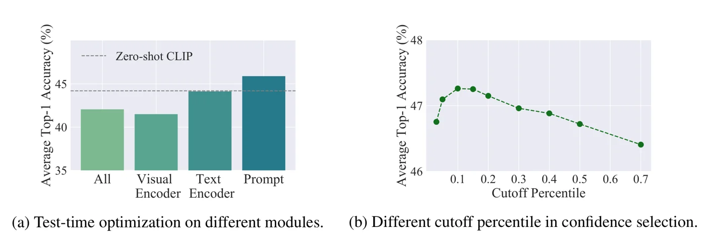 (a) MEMO-style test-time optimisation of different parts of CLIP: only prompt tuning clearly beats zero-shot CLIP (dashed line), the text encoder roughly matches it, and the visual encoder is worst. (b) Cutoff percentile \(\rho\) in confidence selection: accuracy peaks at \(\rho = 0.1\) and falls as more low-confidence views are kept. Figure from the paper.
Panel (a) supports the choice of the prompt as the only parameter to adapt; tuning the full model or the visual encoder on a single image ends below the zero-shot baseline. Panel (b) shows that keeping too few views (\(\rho\) near 0) also hurts, so the cutoff is a trade-off between filtering noisy crops and keeping enough views for a stable average.
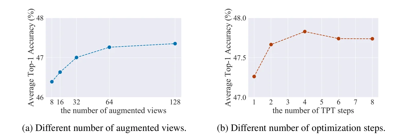 (a) Accuracy rises with the number of augmented views and plateaus around N = 64. (b) Going from 1 to 2 steps adds about 0.4 points, and more steps add almost nothing. Figure from the paper.
These curves are the basis of the default setting (64 views, 1 step): both extra views and extra steps cost inference time roughly linearly, and the gains past those points are small.
Limitations
- Backward pass per test image (stated by the authors). Every prediction needs one optimisation step that backpropagates through the text encoder. In the appendix, inference takes 0.25 s/iter versus 0.10 s/iter for hand-crafted prompts.
- Memory from augmentations (stated by the authors). Each image becomes a batch of 64 views, which increases inference memory.
- More steps give little. Going from 1 to 2 steps adds about 0.4% accuracy, and more steps add almost nothing, while cost grows linearly. Accuracy also drops with fewer views, though 8 views still give over 2% gain on RN50.
- No calibration analysis. The objective drives the model toward confident predictions, but the paper reports only accuracy. Later work (C-TPT) shows that TPT raises expected calibration error substantially.
- Hand-picked settings. \(\rho\), the step count, the learning rate, and the augmentation type are chosen on validation splits (ImageNet validation for the OOD sets, the datasets’ validation splits for the fine-grained sets). Different augmentations are used for the two benchmark groups.
- Not uniformly better. On some fine-grained datasets, CoCoOp or the prompt ensemble is ahead (for example Flower102, Pets, and EuroSAT with ViT-B/16).