Abstract
Point-cloud classifiers lose accuracy under corruptions such as noise, density changes, occlusion and LiDAR-style sparsity. At the time of this paper there were few TTA methods for 3D classification. MATE is really test-time training, since it needs a masked-autoencoder objective during pretraining. BFTT3D keeps a memory of source prototypes, so it is not fully source-free. TENT works on any pretrained model but adapts on a single view of each batch, which can push the model into sharp, unstable solutions.
The paper borrows the idea of weight averaging from SWA and SWAD, where averaging weights along training tends to land in flatter minima. Here the diversity does not come from training steps but from the input: the same point cloud is tokenized several times with different FPS/KNN samplings. TENT is run on each sampling, and the resulting normalization parameters are averaged. The paper does not name the method; this post calls it SVWA, after the authors’ code repository.
Motivation
The gap the paper points to is about the setting more than about accuracy. In 2D, fully test-time adaptation (a model trained normally, then adapted only on unlabeled test data) is well studied, with entropy minimization (TENT, SHOT) and BN-statistics updates as the standard tools. For 3D point-cloud classification the authors count only two TTA methods, and neither fits that setting: MATE changes source pretraining by adding a masked-autoencoder branch, which makes it test-time training, and BFTT3D carries a memory of source prototypes into adaptation. A method that works on an off-the-shelf pretrained classifier with no source data was missing.
The second observation is about how such a method should adapt. TENT updates the normalization layers from a single view of each test batch, and an entropy objective on one view can settle in a sharp minimum that overfits the noise of that batch. SWA and SWAD showed that averaging weights from several points of an optimization trajectory lands in flatter, more robust minima. The key insight is that point clouds offer a cheap, label-free source of diversity for this: FPS and KNN tokenization is stochastic, so the same object can be re-sampled into several slightly different patch sets that keep its global shape. Adapting on each sampling and averaging the resulting weights gives SWAD-style averaging without a training trajectory. The paper has no pilot figure for this argument; the augmentation ablation in Main Experiments is the closest evidence that sampling variation, rather than generic augmentation, is the useful source of diversity.
Method
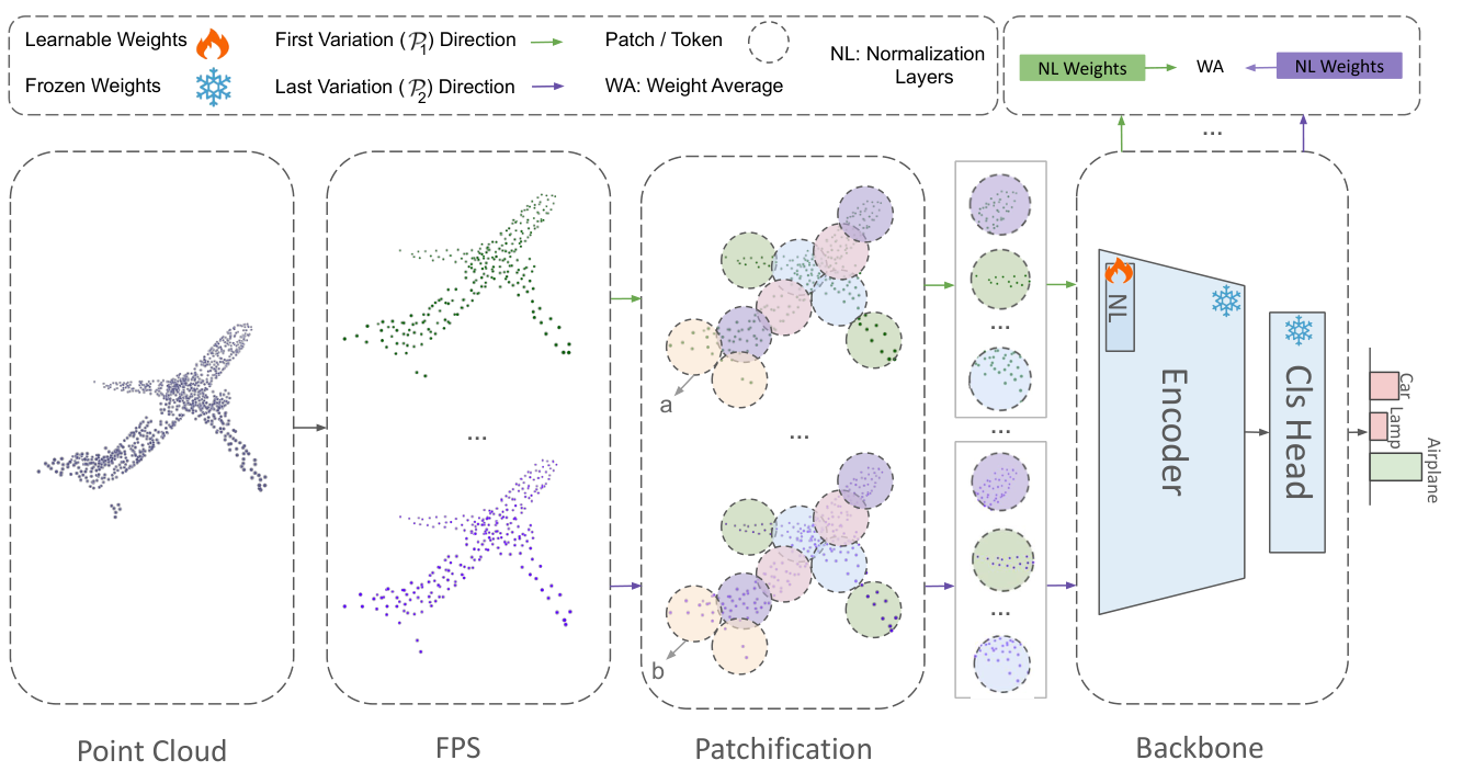 The input point cloud is sampled several times with FPS and patchified with KNN (patches a and b differ between samplings). Only the normalization layers (NL) are trainable. They are adapted with TENT separately for each sampling, and the adapted NL weights are averaged (WA). Figure 1 from the paper.
Sampling variation
A point cloud is \(P \in \mathbb{R}^{N^p \times 3}\). Patch centers are chosen with Farthest Point Sampling:
\[c_i = \arg\max_{p \in P} \min_{c_j \in \{c_1, \dots, c_{i-1}\}} \|p - c_j\|_2 .\]Each center gets a patch of its \(K\) nearest neighbours:
\[P_i = \Bigl\{ p \in P \mid p \in \mathrm{KNN}(c_i) \Bigr\},\]giving \(\mathcal{P} \in \mathbb{R}^{N \times K \times 3}\). FPS depends on its starting point, so running it again with different centers and neighbours gives \(N^V\) versions \(\{\mathcal{P}_1, \dots, \mathcal{P}_V\}\) of the same object. Each version changes local patch geometry slightly but keeps the global shape. For non-Transformer backbones (PointNet, DGCNN) they set \(K = 1\), so each “patch” is just an FPS-selected point.
TENT on each variation
For each \(\mathcal{P}_v\), only the normalization parameters \(\gamma, \beta\) are updated, by minimizing the prediction entropy \(\mathcal{H}\) as in TENT:
\[\gamma^*_i, \beta^*_i = \arg\min_{\gamma, \beta} \mathbb{E}\left[ \mathcal{H}\left( f_\theta(\mathcal{P}_v) \right) \right].\]All other weights stay frozen. For Point-MAE both BN and LN layers are adapted; PointNet and DGCNN only have BN.
Weight averaging
After adapting on each variation, the weights \(\theta_v\) are stored and averaged:
\[\theta_{\text{avg}} = \frac{1}{N^V} \sum_{v=1}^{V} \theta_v .\]The motivation is the flat-minima argument from SWAD’s robust risk minimization, \(\hat{\mathcal{E}}^\gamma_{\mathcal{D}}(\theta) = \max_{\|\Delta\| \le \gamma} \hat{\mathcal{E}}_{\mathcal{D}}(\theta + \Delta)\). The paper does not optimize this objective. It argues that averaging models adapted on different samplings lands in a flatter region and smooths out errors from any single adaptation.
Parallel implementation
In the default “parallel” mode the model is reset before each variation, so the \(N^V\) adaptations are independent. Since only normalization parameters change, the backbone is shared and the \(N^V\) copies of \((\gamma, \beta)\) live inside one “weight average normalization layer”. Defaults are \(N^V = 6\), one TENT iteration, AdamW with learning rate \(10^{-3}\), and batch size 128 for Point-MAE and PointNet.
Main Experiments
Top-1 accuracy (%), mean over 15 corruptions, from Tables 1-3 (the paper also lists every corruption). Three backbones: Point-MAE, PointNet, DGCNN. This is a subset of the baselines: the strongest source-free ones plus BFTT3D. Results marked * were not reproduced by the authors; all others were. † uses source data during adaptation. “-“ means the paper has no entry.
| Backbone | Method | ModelNet40-C | ShapeNet-C | ScanObjectNN-C |
|---|---|---|---|---|
| Point-MAE | Source-Only | 53.9 | 61.3 | 33.1 |
| MATE* | 64.3 | 63.1 | 47.0 | |
| PL | 71.0 | 66.2 | 45.8 | |
| MEMO | 69.4 | 42.3 | 46.1 | |
| TENT | 72.1 | 66.1 | 45.9 | |
| Ours | 75.0 | 67.0 | 46.1 | |
| PointNet | Source-Only | 46.5 | 49.8 | 29.7 |
| PL | 59.6 | 54.3 | 39.5 | |
| BFTT3D† | 66.2 | - | 45.5 | |
| MEMO | 58.5 | 28.0 | 40.2 | |
| TENT | 60.4 | 55.5 | 39.7 | |
| Ours | 61.3 | 56.9 | 40.6 | |
| DGCNN | Source-Only | 58.8 | 63.6 | 37.9 |
| PL | 70.7 | 67.0 | 48.1 | |
| BFTT3D† | 70.7 | - | 56.1 | |
| MEMO | 63.5 | 28.7 | 45.0 | |
| TENT | 71.6 | 67.0 | 48.3 | |
| Ours | 74.2 | 66.0 | 49.9 |
The method beats TENT in 8 of 9 backbone-dataset pairs. The clearest gains are on ModelNet40-C (+2.9 with Point-MAE, +2.6 with DGCNN). Elsewhere the margins are often under one point, and on ShapeNet-C with DGCNN it is one point below TENT. BFTT3D is higher on PointNet and on DGCNN/ScanObjectNN-C, but it uses source prototypes. In the ablations, accuracy on ModelNet40-C with Point-MAE rises from about 74.0% to 76.0% as \(N^V\) goes from 2 to 12, and replacing sampling variation with flips or rotations hurts, sometimes below Source-Only.
The full per-corruption table for ModelNet40-C shows that the Point-MAE gain over TENT is spread across almost every corruption, with the largest jumps on upsampling (78.2 to 87.0), LiDAR (51.2 to 55.3), and background noise (26.7 to 33.0). For PointNet and DGCNN the wins are more mixed, and TENT is still better on several corruptions.
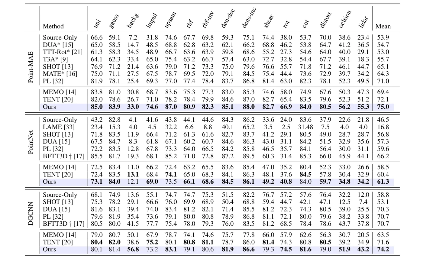 Table 1 of the paper: top-1 accuracy on each of the 15 ModelNet40-C corruptions for Point-MAE, PointNet, and DGCNN. “Ours” (highlighted) is best on most Point-MAE columns; with the other backbones the margin over TENT is smaller and not uniform. Figure from the paper.
Two ablations on ModelNet40-C with Point-MAE support the design. Accuracy grows steadily with the number of samplings \(N^V\), and when the same weight-averaging pipeline is driven by standard augmentations instead of re-sampling, horizontal flips and rotations fall below Source-Only (53.95), jitter reaches 68.97, and sampling variation reaches 75.03.
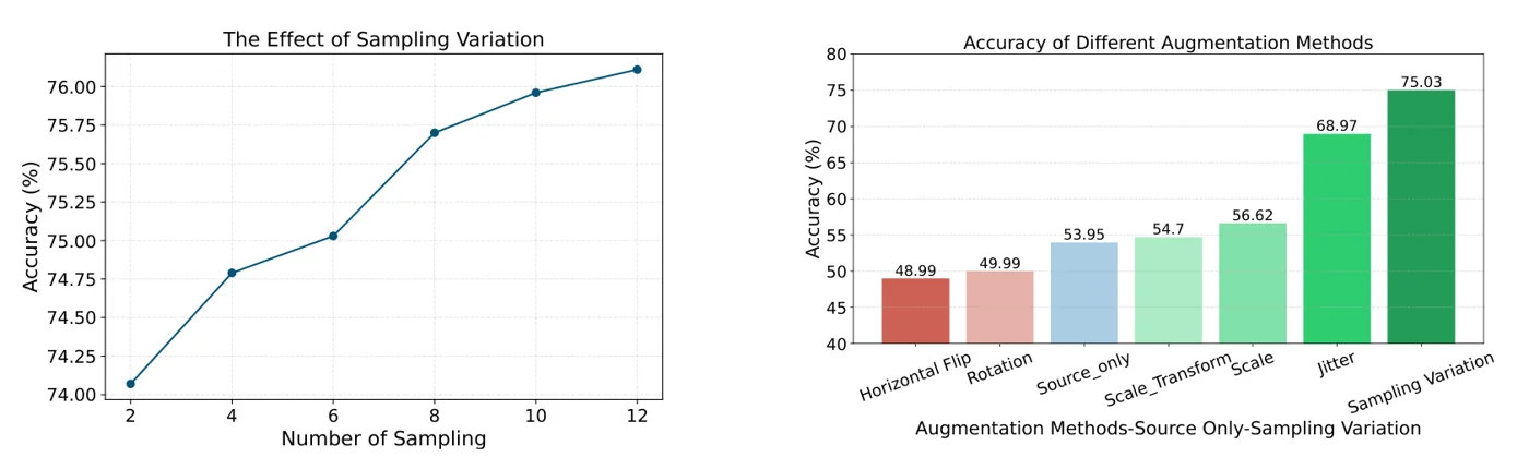 Left: accuracy vs. the number of samplings \(N^V\) (about 74.1% at 2, 76.1% at 12). Right: the weight-averaging pipeline with different sources of variation; only jitter and sampling variation beat Source-Only by a wide margin. Batch size 128, one iteration. Figure from the paper.
The gap over TENT also holds across batch sizes and numbers of adaptation steps. At batch size 8 the method is at about 69% against about 66% for TENT, and with more iterations both improve while the gap stays around 3 points.
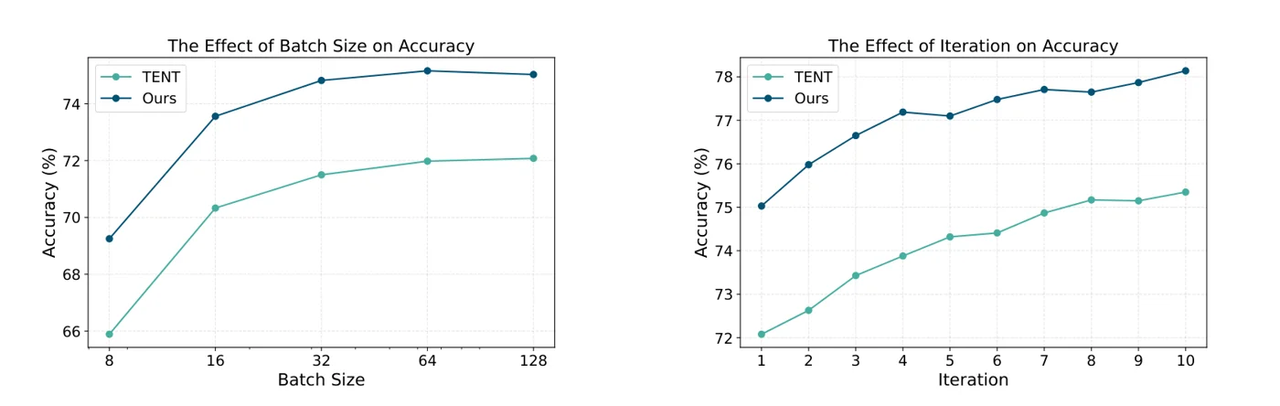 Accuracy of TENT and the method (“Ours”) on ModelNet40-C with Point-MAE as the batch size (left, 8 to 128) and the number of iterations (right, 1 to 10) change. The method stays above TENT throughout. Figure from the paper.
Limitations
- The paper has no limitations section.
- It still needs backpropagation, and it runs \(N^V\) forward and backward passes per batch. With \(N^V = 6\) on PointNet, the reported adaptation time is about 26 ms versus 21 ms for TENT, and memory overhead is about 1.8%. These numbers are only given for PointNet in parallel mode.
- The default batch size is large (128 for Point-MAE and PointNet). The batch-size ablation shows the gain over TENT holds down to batch size 8, but only on ModelNet40-C with Point-MAE.
- The gains over TENT are small on many settings and negative on ShapeNet-C with DGCNN, so the benefit is not uniform across backbones and datasets.
- The flat-minima explanation is by analogy. The paper does not measure flatness or optimize the robust risk.
- Sampling variation relies on FPS/KNN tokenization. For PointNet and DGCNN it reduces to choosing different FPS subsets.