Abstract
MATE showed that test-time training (TTT) for 3D point clouds works if the network reconstructs each masked test sample before classifying it. The authors point out two problems. First, MATE reconstructs surface points, so its features stay sensitive to surface-level corruptions such as noise. Second, it updates all network parameters with backpropagation at test time, which keeps its frame rate low.
SMART-PC swaps the reconstruction task for skeleton prediction. Each patch predicts a sphere (a skeletal point and a radius) that summarizes the local shape. This abstraction averages out high-frequency noise, so the encoder learns features that hold up better under corruption. With such features, online adaptation can skip backpropagation and only update the BatchNorm running mean and variance.
Motivation
The paper starts from MATE, the main TTT method for 3D point clouds, and names two weaknesses. The first is what its self-supervised task teaches. MATE reconstructs masked surface points, so the encoder is trained to model exactly the surface details that corruptions such as noise, dropout, or LiDAR sparsity damage. Features built to reproduce the surface stay sensitive to it. The second is cost. MATE adapts by backpropagating through all network parameters for every test sample, which keeps it near 10 frames per second and far from real-time use.
The key insight is to change the pretext task so that the features become robust enough that adaptation no longer needs gradients. A skeleton, a set of spheres whose centers lie inside the shape and whose radii reach its surface, is an abstraction of the geometry: it keeps the overall structure and averages out high-frequency noise and local distortions. If the encoder is trained to predict skeletons instead of surfaces, the authors argue, its features depend on the underlying shape, and a cheap update of the BatchNorm statistics is enough to follow the shift, as in 2D work on BN adaptation.
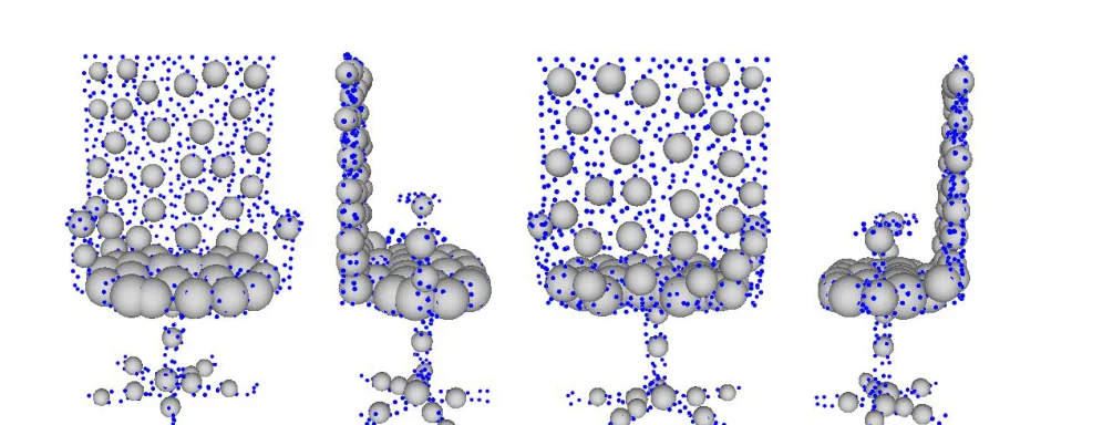 Chair point clouds seen from the front and the side: gray spheres are skeletal points drawn with their radii, blue dots are points sampled on the sphere surfaces. A few dozen spheres capture the seat, back, and legs. Figure from the paper.
Method
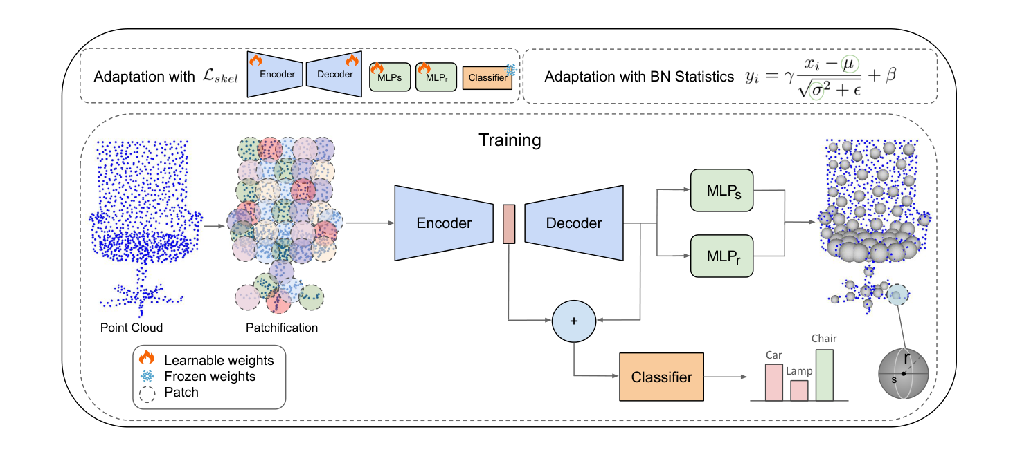 SMART-PC: a shared Point-MAE encoder-decoder feeds two MLPs that predict skeletal sphere centers and radii, and a classifier that takes the sum of encoder and decoder features. At test time the model adapts either with the skeletal loss and backpropagation, or by updating BatchNorm statistics only. Figure from the paper.
Patchification
A point cloud \(P\in\mathbb{R}^{N\times 3}\) is split into patches. Farthest point sampling picks \(M\) centers, and each center takes its \(K\) nearest neighbors:
\[C = \mathit{FPS}(P)\in\mathbb{R}^{M\times 3}, \qquad P_{local} = \mathit{kNN}(C,P)\in\mathbb{R}^{M\times K\times 3}\]Skeletal branch
A skeletal sphere is \(s=\big(c_s, r(c_s)\big)\in\mathbb{R}^4\): a center \(c_s\) and a radius \(r(c_s)\) that reaches the shape surface. Any point on the sphere is \(p = c_s + r(c_s)\cdot v\) for a unit vector \(v\), so a set of spheres can describe the whole shape.
The encoder and decoder process the patches, and two MLPs predict one sphere per patch:
\[F_{enc}=E(P_{local}), \quad F_{dec}=D(F_{enc}), \quad c_s=\mathit{MLP}_s(F_{dec})\in\mathbb{R}^{M\times 3}, \quad r=\mathit{MLP}_r(F_{dec})\in\mathbb{R}^{M\times 1}\]Earlier skeleton methods such as Point2Skeleton build skeletal points as convex combinations of input points. SMART-PC predicts them directly from features. The authors argue that feeding raw points into the prediction makes the task too easy and keeps the encoder from learning robust features.
Classification branch
The classifier uses the sum of encoder and decoder features, so it also sees the skeleton-related decoder features:
\[F_{combined} = F_{enc} + F_{dec}, \qquad p = \mathit{Softmax}\big(\mathit{MLP}_{cls}(F_{combined})\big)\]Training losses
The skeletal branch is self-supervised with three losses. The point-to-sphere loss pulls input points onto sphere surfaces and spheres toward input points:
\[\mathcal{L}_{p2s} = \sum_{p\in P}\Big(\min_{s\in S}\|p-c_s\|_2 - r(c_s)\Big) + \sum_{s\in S}\Big(\min_{p\in P}\|c_s-p\|_2 - r(c_s)\Big)\]The sampling loss is a Chamfer distance between the input \(P\) and points \(T\) sampled on the sphere surfaces. The radius loss \(\mathcal{L}_{radius} = -\sum_{s\in S} r(c_s)\) pushes radii to be larger, so each sphere covers a wider region and single noisy points matter less. The total loss is
\[\mathcal{L}_{total} = \underbrace{\mathcal{L}_{p2s} + \lambda_1\mathcal{L}_{sampling} + \lambda_2\mathcal{L}_{radius}}_{\mathcal{L}_{skel}} + \mathcal{L}_{cls}\]where \(\mathcal{L}_{cls}\) is cross entropy on the labeled source data. The best coefficients in the ablation follow Point2Skeleton.
Test-time adaptation
The top row of the figure shows the two adaptation options. Both follow MATE’s protocol (batch size 1, with the sample copied into a batch of augmented views, here random rotations instead of random masks).
- Online, BatchNorm only (marked †): the model is not reset between samples, only between corruption types. No gradients are computed. Only the BatchNorm running mean \(\mu\) and variance \(\sigma^2\) are updated with target data, in \(y_i = \gamma \frac{x_i-\mu}{\sqrt{\sigma^2+\epsilon}} + \beta\).
- Online or Standard with \(\mathcal{L}_{skel}\): the encoder, decoder and skeletal MLPs are updated by backpropagating the skeletal loss, with the classifier frozen. Standard mode resets the model after each batch and runs 20 iterations, so BatchNorm statistics alone would not help there.
Main Experiments
Backbone: Point-MAE. Metric: mean top-1 accuracy (%) over 15 corruptions. Batch size 1, one iteration (online) or 20 iterations (standard). Copied from Table 1; the paper’s differences against MATE are left out. * marks results the authors reproduced, † marks backpropagation-free adaptation, ‡ marks diffusion-based methods.
| Method | ModelNet-40C | ScanObjectNN-C | ShapeNet-C |
|---|---|---|---|
| Org-SO* | 54.0 | 37.0 | 61.3 |
| MATE-SO* | 54.4 | 34.5 | 56.5 |
| SMART-PC-SO | 61.7 | 38.7 | 64.5 |
| DUA | 54.7 | 38.7 | 60.8 |
| TTT-Rot | 53.0 | – | 60.9 |
| SHOT | 26.6 | 29.6 | 36.2 |
| T3A | 55.7 | – | 54.4 |
| TENT | 26.5 | 27.7 | 37.4 |
| CloudFixer-Standard‡ | 68.0 | - | - |
| CloudFixer-Online‡ | 77.2 | - | - |
| DDA-Standard‡ | 68.1 | - | - |
| SVWA-Standard* | 57.1 | 37.4 | 50.5 |
| MATE-Standard* | 63.0 | 36.9 | 63.1 |
| SMART-PC-Standard | 63.1 | 39.6 | 64.4 |
| BFTT3D* | 57.2 | 33.0 | 60.7 |
| MATE-Online* | 70.6 | 36.9 | 69.1 |
| SMART-PC-Online† | 70.8 | 46.7 | 65.9 |
| SMART-PC-Online | 72.9 | 47.4 | 67.1 |
Adaptation speed on ModelNet40-C (Table 4, appendix):
| Method | DDA | CloudFixer | BFTT3D | SVWA (Nv=2) | MATE | SMART-PC |
|---|---|---|---|---|---|---|
| FPS | 0.04 | 1.07 | 6.83 | 10.86 | 10.79 | 59.52 |
The clearest gains come before any adaptation: skeleton pre-training alone lifts source-only accuracy by 7.3 points on ModelNet-40C and 8.0 points on ShapeNet-C over MATE-SO. In the standard mode SMART-PC and MATE are close (63.1 vs 63.0 on ModelNet-40C). The BatchNorm-only variant matches MATE-Online on ModelNet-40C and beats it by about 10 points on ScanObjectNN-C at roughly 5.5 times the frame rate, but it trails MATE-Online on ShapeNet-C (65.9 vs 69.1). CloudFixer-Online is still higher on ModelNet-40C (77.2), though it runs at about 1 FPS.
The speed argument is shown directly in the online setting on ScanObjectNN-C. With the BatchNorm-only update, SMART-PC stays at about 46.6% accuracy whether each sample is expanded into 48 or 24 augmented copies, and with 24 copies it passes 30 frames per second. MATE stays near 37% at roughly 8 to 10 FPS, because its per-sample backpropagation dominates the cost.
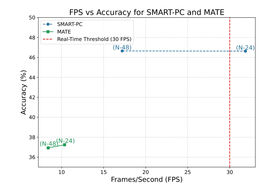 Online adaptation on ScanObjectNN-C with 48 or 24 augmented copies per sample (N-48, N-24). SMART-PC (BatchNorm-only) crosses the 30 FPS real-time line at N-24 with no loss in accuracy; MATE is about 10 points lower and about three times slower. Figure from the paper.
Two ablations look at the adaptation protocol. In online mode on ScanObjectNN-C, SMART-PC reaches 46.42% even without augmentation during adaptation, already well above MATE (36.93%), and rotations add about one point (47.36%). In standard mode on ModelNet40-C, accuracy grows with batch size from 67.94% at 8 to 73.42% at 128, although the main results use batch size 1 to match MATE.
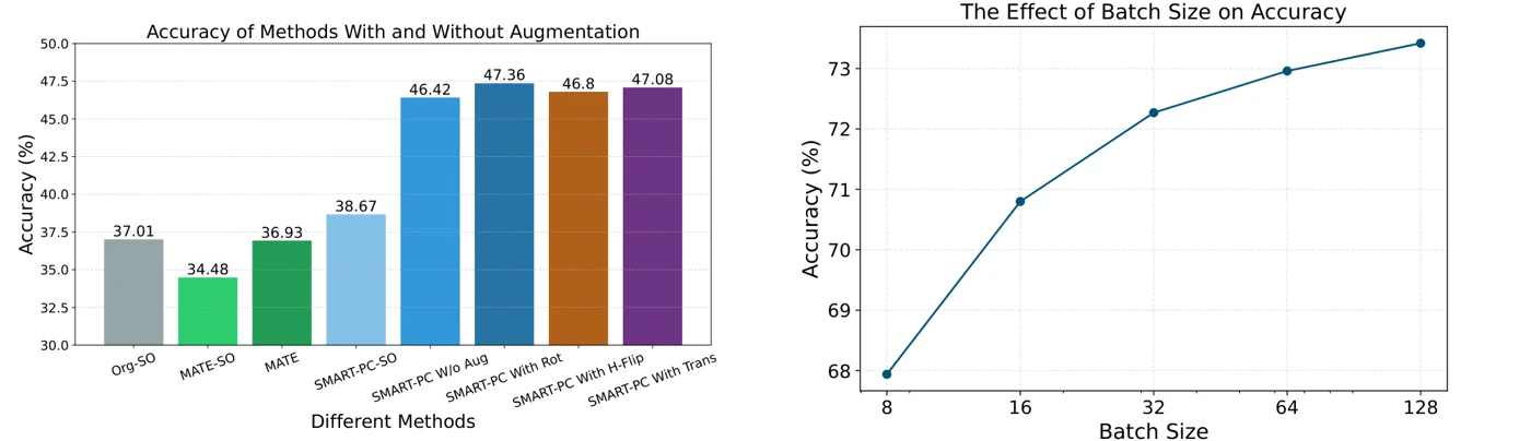 Left: online accuracy on ScanObjectNN-C for the source-only baselines, MATE, and SMART-PC with no augmentation, rotation, horizontal flip, or translation during adaptation. Right: effect of batch size on mean ModelNet40-C accuracy in standard mode. Figure from the paper.
The appendix also visualizes why updating the BatchNorm statistics is enough. On clean data the feature distributions of the first BN layers match the pretrained running statistics. On corrupted data they drift away from them, most visibly in the classifier’s BN layer, and the adapted statistics move back onto the corrupted distributions without any change to the learned weights.
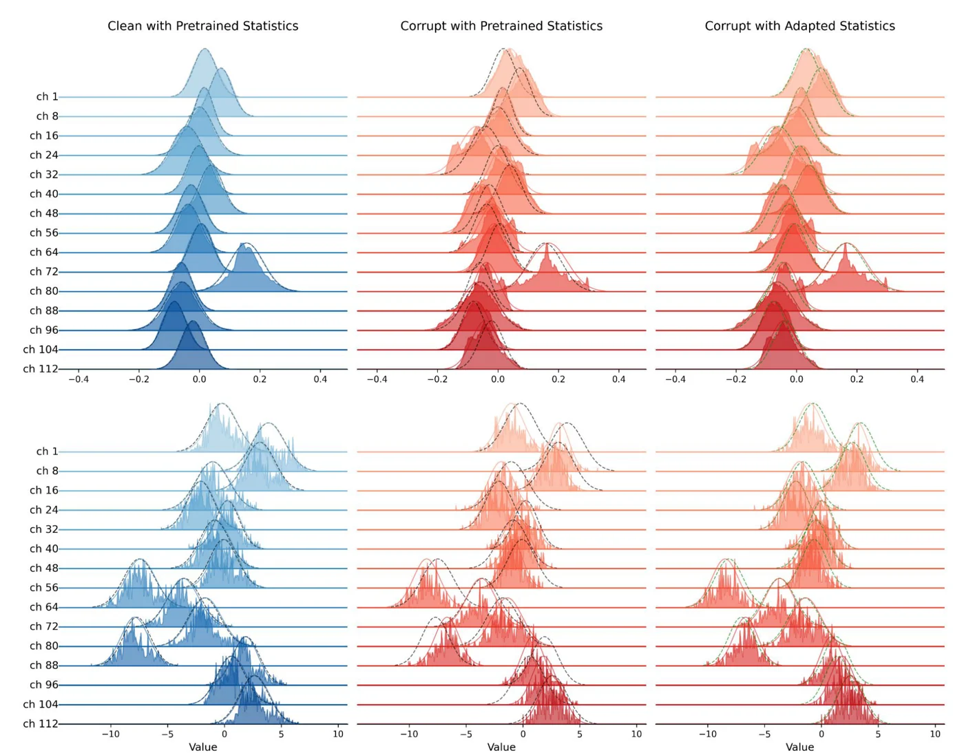 Per-channel input distributions (solid) and BatchNorm running statistics (dashed) for the first BN layer of the encoder (top) and of the classifier (bottom). Blue: clean source data with pretrained statistics. Red: corrupted data with pretrained statistics (black dashed, mismatched) and with adapted statistics (green dashed, matched). Figure from the paper.
Limitations
- The paper has no limitations section. Its conclusion lists other 3D tasks (segmentation, detection) as future work, so only classification is tested.
- It needs a special pre-training stage with the skeletal branch. The BatchNorm-only mode works because of these features, so it does not apply to an arbitrary pretrained model.
- On ShapeNet-C, both online variants are below MATE-Online (67.1 and 65.9 vs 69.1).
- The MATE baselines are reproduced and come out slightly lower than in the MATE paper (MATE-Online 70.6 vs 71.3 on ModelNet-40C; MATE-Standard 63.0 vs 64.3). Against the originally reported 71.3, SMART-PC-Online† (70.8) would no longer be ahead. The text also quotes different MATE numbers than the table in places (53.7 and 69.6).
- Batch size 1 still means 48 or 24 rotated copies of each sample per step, and the BatchNorm-only mode updates running statistics over the stream. It needs a stream of samples to build useful statistics. The protocol also resets the model at each new corruption type, which assumes the shift is known to change at that point. Mixed or continually changing shifts are not tested.
- The speed claim is mainly for the BatchNorm-only online mode. The modes that backpropagate \(\mathcal{L}_{skel}\) through the full model, including the 20-step standard mode, carry a cost similar to MATE.