Abstract
Test-time prompt tuning (TPT) adapts CLIP’s text prompt to each test image by minimising the entropy of the averaged prediction over augmented views. Entropy minimisation makes the model overconfident, so calibration gets worse. C-TPT and O-TPT fix this with a regulariser on the class text embeddings (prototypes). C-TPT spreads them away from their centroid. O-TPT pushes every pair of prototypes toward orthogonality. The authors argue that full orthogonality is too aggressive for classes that really are similar, such as “annual crop land” and “permanent crop land” in EuroSAT. Pulling such pairs apart makes the model confident even when it is wrong.
SoC (Semantic Orthogonal Calibration) keeps the idea of separating prototypes but uses a Huber penalty on pairwise cosine similarity. The penalty is quadratic for small similarities and linear for large ones, so the repulsion between very similar classes is capped. The paper backs this with a confidence lower bound in terms of the largest pairwise similarity and a one-step analysis showing that O-TPT shrinks that similarity faster than SoC.
Motivation
The starting point is a failure case of the calibration fix rather than of TPT itself. Entropy minimization makes TPT overconfident, and C-TPT and O-TPT counter this by spreading the class text prototypes apart. O-TPT goes furthest and asks for every pair to be orthogonal. The authors argue that this ignores the fact that some classes really are semantically close. In EuroSAT, an “annual crop land” image is easily confused with “permanent crop land”. Zero-shot CLIP gets such an image wrong but stays uncertain, splitting its softmax between the two classes. O-TPT pushes the two prototypes apart, so the same wrong prediction becomes confident (the teaser figure in the Method section shows this example).
The paper backs the example with an analysis on EuroSAT. For every ordered class pair \((i, j)\) it takes the wrong predictions (predicted \(i\), true label \(j\)), computes their ECE, and plots it against the zero-shot cosine similarity of the two class prototypes. For O-TPT, ECE grows with similarity (correlation \(r=+0.69\)), and the most similar pairs, which also hold the most samples, have ECE near 90. SoC removes this trend (\(r=-0.20\)).
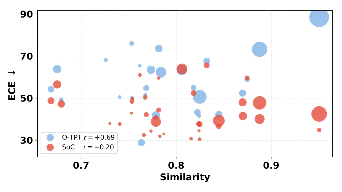 ECE of the wrong predictions for each class pair on EuroSAT, against the zero-shot cosine similarity of the pair. Circle size is the number of samples. O-TPT (blue) is most overconfident on the most similar pairs; SoC (red) is not. Figure from the paper.
The key insight is that the repulsion between prototypes should depend on how similar they are: strong enough to undo the collapse caused by entropy minimization, but capped for pairs that are similar for a real semantic reason. A Huber penalty on the pairwise cosine similarity does exactly this, and the paper’s confidence bound and one-step analysis make the argument formal.
Method
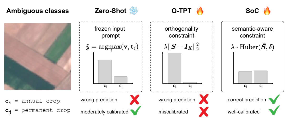 Motivating example on EuroSAT. Zero-shot CLIP is wrong but uncertain between two close classes. O-TPT’s orthogonality constraint makes it wrong and confident. SoC’s semantic-aware Huber constraint keeps the two classes close in confidence. Figure from the paper.
The paper has no separate architecture diagram. SoC is a one-term change to the TPT loss, and the figure above shows the effect it targets.
Setting
CLIP gives an image embedding \(\mathbf{v}\) and class prototypes \(\mathbf{t}_k = f_\phi(\text{"a photo of a [CLASS]"})\), all unit norm. Logits are \(z_k = \alpha\,\mathbf{v}^\top \mathbf{t}_k\) with CLIP’s learned scale \(\alpha\). Stacking the prototypes in \(\mathbf{E} \in \mathbb{R}^{K\times d}\) gives the similarity matrix \(\mathbf{S} = \mathbf{E}\mathbf{E}^\top\) with entries \(s_{ij} = \mathbf{t}_i^\top \mathbf{t}_j\). The two baselines add a regulariser to the TPT entropy loss:
\[\mathcal{L}_{\text{C-TPT}} = \mathcal{L}_{\text{TPT}} - \lambda \frac{1}{K}\sum_{k=1}^{K} \|\bar{\mathbf{t}} - \mathbf{t}_k\|_2, \qquad \mathcal{L}_{\text{O-TPT}} = \mathcal{L}_{\text{TPT}} + \lambda \|\mathbf{S} - \mathbf{I}_K\|_2^2 .\]The SoC regulariser
O-TPT’s penalty is quadratic in \(s_{ij}\), so its gradient grows with the similarity. The most similar pairs get pushed hardest. SoC uses a Huber function with margin \(\delta \in [0,1]\):
\[\mathcal{L}_{\text{Huber}}(s,\delta) = \begin{cases} \frac{s^2}{2} & \text{if } s \le \delta \\ \delta\left(s - \frac{\delta}{2}\right) & \text{otherwise} \end{cases}\] \[\mathcal{L}_{\text{SoC}} = \mathcal{L}_{\text{TPT}} + \lambda \cdot \frac{2}{K(K-1)} \sum_{i<j} \mathcal{L}_{\text{Huber}}(s_{ij}, \delta).\]The gradient with respect to \(\mathbf{t}_i\) is \(\sum_{k\neq i} g_\delta(s_{ik})\,\mathbf{t}_k\) with \(g_\delta(s) = \min(s, \delta)\). So pairs above the margin all receive the same, bounded push.
In practice the similarities are min-max normalised, \(\tilde{\mathbf{S}} = (\mathbf{S} - \mathbf{S}_{\min}) / (\mathbf{S}_{\max} - \mathbf{S}_{\min})\), and \(\delta\) is set to the 20th percentile of \(\tilde{\mathbf{S}}\) for each dataset. The weight is \(\lambda = 30\) (14 for the ImageNet shift experiments), rescaled by the ratio of the two loss magnitudes.
Why this should help calibration
With \(\mu = \max_{i\neq j} \mathbf{t}_i^\top \mathbf{t}_j\) (the worst-case similarity), Proposition 1 gives a floor on the top softmax probability for any unit \(\mathbf{v}\):
\[p_{\max}(\mathbf{v}) \ge \frac{1}{1 + (K-1)\exp(-\alpha(1-\mu))}.\]Lower \(\mu\) means a higher confidence floor. TPT methods take a single gradient step. Keeping only the most similar pair and using a first-order expansion, one step of size \(\eta\) gives
\[\mu'_{\text{O-TPT}} \approx (1-4\eta)\mu, \qquad \mu'_{\text{Huber}} \approx \begin{cases} (1-2\eta)\mu & \mu \le \delta \\ \mu - 2\eta\delta & \mu > \delta . \end{cases}\]O-TPT reduces \(\mu\) more in both regimes, so it raises the confidence floor more (Corollary 1). The authors connect this to the overconfidence of O-TPT on semantically close class pairs, which they show as per-pair ECE against zero-shot similarity on EuroSAT.
Main Experiments
Setup: CLIP ViT-L/14 unless stated, prompt initialised as “a photo of a”, one AdamW step with lr 0.005, 64 augmented views per image. Metrics are top-1 accuracy (%) and ECE (%). The “11 datasets” average covers ImageNet plus the 10 fine-grained and specialised datasets (DTD, Flowers, Food101, SUN397, Aircraft, Pets, Caltech, UCF101, EuroSAT, Cars). The table below collects only the average columns from the paper’s Tables 1, 2 and 3.
| Method | 11 datasets, ViT-L/14 Acc | ECE | 11 datasets, ViT-B/16 Acc | ECE | ImageNet-A/v2/R/Sketch, ViT-L/14 Acc | ECE |
|---|---|---|---|---|---|---|
| Zero-Shot | 71.1 | 5.1 | 63.9 | 4.2 | 70.0 | 4.4 |
| TPT | 72.0 | 14.9 | 65.2 | 11.2 | 72.9 | 14.2 |
| C-TPT | 72.1 | 10.0 | 64.6 | 5.0 | 72.0 | 12.6 |
| O-TPT | 71.4 | 7.7 | 64.0 | 4.8 | 71.3 | 9.9 |
| SoC | 72.3 | 5.4 | 64.6 | 4.3 | 71.3 | 8.4 |
Per-dataset ECE with ViT-L/14 (paper’s Table 1), SoC vs. O-TPT:
| Method | ImgNet | DTD | Flowers | Food101 | SUN397 | Aircraft | Pets | Caltech | UCF101 | EuroSAT | Cars |
|---|---|---|---|---|---|---|---|---|---|---|---|
| O-TPT | 5.5 | 13.8 | 7.0 | 2.8 | 7.6 | 16.8 | 1.4 | 2.0 | 8.5 | 17.7 | 2.2 |
| SoC | 7.2 | 10.9 | 5.3 | 2.1 | 7.2 | 12.7 | 0.5 | 1.3 | 6.5 | 3.2 | 2.2 |
SoC has the lowest average ECE among the adapted methods in every setting, and with ViT-L/14 its ECE (5.4) is close to zero-shot CLIP (5.1) while its accuracy is slightly higher. The largest single change is EuroSAT, where ECE drops from 17.7 to 3.2 and accuracy rises from 53.6 to 58.3. Under the ImageNet shifts, accuracy equals O-TPT and stays below TPT and C-TPT. With two gradient steps instead of one, SoC’s ECE degrades by about 23% versus 39% for O-TPT, which matches the one-step analysis.
The reliability diagrams on three datasets show where the ECE gain comes from. O-TPT’s bars sit below the diagonal in the high-confidence bins, which is overconfidence. With SoC the bars move closer to the diagonal, most clearly on EuroSAT (ECE 17.7 to 3.2), while Aircraft remains overconfident (16.8 to 12.7).
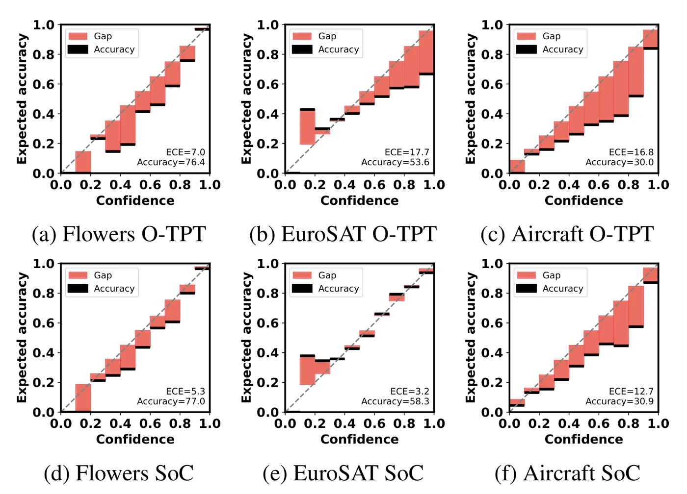 Reliability diagrams for O-TPT (top) and SoC (bottom) on Flowers102, EuroSAT, and FGVC Aircraft, with ECE and accuracy in each panel. SoC is closer to the diagonal on all three, with the biggest change on EuroSAT. Figure from the paper.
The two-step experiment tests the one-step analysis directly. Taking a second gradient step raises ECE for all three regularizers, but by +44.2% for C-TPT, +39.2% for O-TPT, and +22.8% for SoC, while accuracy changes by less than one point.
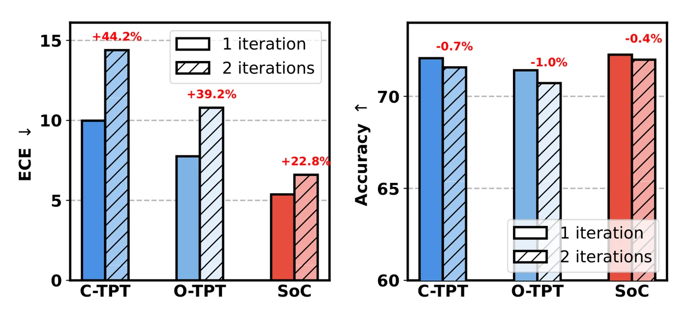 Average ECE (left) and accuracy (right) over 11 datasets for C-TPT, O-TPT, and SoC with one (solid) and two (hatched) gradient steps. The relative ECE increase is smallest for SoC. Figure from the paper.
Calibration also depends on the initial prompt. Over 18 CLIP prompt templates, SoC has lower ECE than O-TPT for every template on DTD and for most templates on Aircraft, so the gain does not depend on the choice of “a photo of a”.
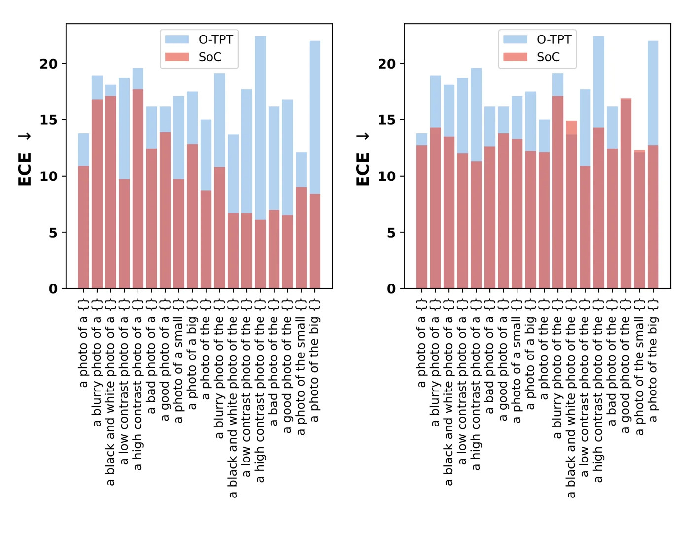 ECE on DTD (left) and Aircraft (right) for O-TPT (blue) and SoC (red) with 18 different initial prompt templates from CLIP. SoC is lower on almost every prompt, and O-TPT’s worst cases (above 20) disappear. Figure from the paper.
Limitations
- Accuracy is not the gain. On the ImageNet variants SoC matches O-TPT (71.3) and trails TPT (72.9) and C-TPT (72.0). With ViT-B/16 it trails TPT (64.6 vs. 65.2).
- Not better everywhere. SoC’s ECE on ImageNet is worse than O-TPT (7.2 vs. 5.5), and it ties on Cars.
- One dataset carries much of the average. EuroSAT accounts for a 14.5-point ECE drop out of 11 datasets. On the other ten datasets the ECE difference to O-TPT is at most 4.1 points.
- Simplified theory. The analysis keeps only the most similar pair, uses a first-order expansion of one gradient step, and gives a lower bound on confidence. It explains a direction of change, not the size of the calibration error.
- Extra choices. The margin is a per-dataset percentile of min-max normalised similarities, \(\lambda\) differs between benchmarks (30 vs. 14), and the loss is rescaled by the ratio of loss magnitudes. The appendix ablates \(\lambda\) on four datasets, but no ablation of the percentile used for \(\delta\) is reported.
- Still bound to TPT’s cost. SoC keeps TPT’s per-image optimisation with 64 augmented views. Its regulariser costs \(O(n^2)\) in the number of classes versus \(O(n^3)\) for O-TPT, but the main inference cost is unchanged.