- PyTorch for Deep Learning (Daniel Bourke, freeCodeCamp) Chapter 4 정리
- 교재: learnpytorch.io
- 코드: MIT License
지난 글에서 피자, 스테이크, 초밥 이미지 폴더를 ImageFolder와 직접 만든 Dataset으로 불러왔다. 이 글은 지난 글의 data_path, image_path, image_path_list, train_dir, test_dir, plot_transformed_images(), device를 그대로 쓴다.
데이터 증강
변환(transform)은 이미지를 어떤 식으로든 바꾼다. 텐서로 바꾸는 것도 변환이고, 자르기, 일부를 무작위로 지우기, 무작위로 회전하기도 변환이다. 이 중 학습 데이터를 바꾸는 변환을 흔히 데이터 증강(data augmentation) 이라 한다.
데이터 증강은 학습 세트의 다양성을 인위적으로 늘리는 과정이다. 이렇게 바뀐 데이터로 학습한 모델은 더 잘 일반화(generalization) 하기를, 즉 처음 보는 예시에도 더 강건한 패턴을 배우기를 기대한다. torchvision.transforms의 다양한 증강 예는 PyTorch의 Illustration of Transforms에서 볼 수 있다.
머신러닝은 무작위성의 힘을 활용하는 분야이며, 연구에 따르면 transforms.RandAugment()나 transforms.TrivialAugmentWide() 같은 무작위 변환이 사람이 고른 변환보다 대체로 낫다. TrivialAugment의 아이디어는 이름처럼 단순하다. 변환 목록에서 무작위로 하나를 골라, 주어진 범위 안의 무작위 강도(magnitude)로 이미지에 적용한다. PyTorch 팀도 최신 비전 모델을 학습할 때 이것을 썼다.
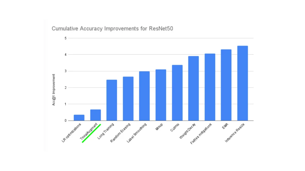 ResNet50의 누적 정확도(Acc@1) 향상. 학습률 최적화, TrivialAugment(초록 밑줄), 더 긴 학습, Random Erasing, Label Smoothing, Mixup, Cutmix, Weight Decay, FixRes, EMA, Inference Resize를 차례로 더할 때마다 향상폭이 쌓여 마지막에는 약 4.5%p에 이른다. 출처: learnpytorch.io (Daniel Bourke, MIT License).
그래프의 막대는 왼쪽부터 기법을 하나씩 추가했을 때의 누적 향상이다. 학습률 최적화만으로는 약 0.3%p, TrivialAugment를 더하면 약 0.7%p가 되어, 단독으로 0.3%p 정도를 보탠다. 여러 작은 기법이 쌓여 최신 성능을 만든다는 것을 보여 준다.
transforms.TrivialAugmentWide()에서 눈여겨볼 인자는 num_magnitude_bins=31이다. 변환 강도를 고르는 범위를 정하며, 0이면 범위가 없고 31이면 범위가 최대다(가장 강한 강도가 나올 가능성이 가장 높다).
from torchvision import transforms

train_transforms = transforms.Compose([
    transforms.Resize((224, 224)),
    transforms.TrivialAugmentWide(num_magnitude_bins=31),  # 증강 강도 범위
    transforms.ToTensor()  # 마지막에 두어 모든 값을 0~1로
])

# 테스트 데이터에는 증강하지 않는다
test_transforms = transforms.Compose([
    transforms.Resize((224, 224)),
    transforms.ToTensor()
])
테스트 세트에는 보통 증강을 하지 않는다. 증강의 목적은 학습 세트의 다양성을 늘려 테스트 세트를 더 잘 예측하는 것이기 때문이다. 다만 테스트 이미지도 텐서로 바꾸고, 보통 학습 이미지와 같은 크기로 맞춘다.
plot_transformed_images(image_paths=image_path_list,
                        transform=train_transforms,
                        n=3,
                        seed=None)
여러 번 실행할 때마다 같은 원본이 다른 모습(색 반전, 기울임, 밝기 변화 등)으로 바뀐다.
Model 0: 증강 없는 TinyVGG
먼저 증강 없이, 크기만 64×64로 맞추고 텐서로 바꾸는 단순한 변환으로 기준 모델을 만든다.
변환과 데이터 불러오기
import os
import torch
from torch import nn
from torchvision import datasets
from torch.utils.data import DataLoader

simple_transform = transforms.Compose([
    transforms.Resize((64, 64)),
    transforms.ToTensor(),
])

# 1. 폴더 -> Dataset
train_data_simple = datasets.ImageFolder(root=train_dir, transform=simple_transform)
test_data_simple = datasets.ImageFolder(root=test_dir, transform=simple_transform)

# 2. Dataset -> DataLoader
BATCH_SIZE = 32
NUM_WORKERS = os.cpu_count()  # 사용 가능한 CPU 코어를 모두 데이터 로딩에
print(f"Creating DataLoader's with batch size {BATCH_SIZE} and {NUM_WORKERS} workers.")

train_dataloader_simple = DataLoader(train_data_simple, batch_size=BATCH_SIZE,
                                     shuffle=True, num_workers=NUM_WORKERS)
test_dataloader_simple = DataLoader(test_data_simple, batch_size=BATCH_SIZE,
                                    shuffle=False, num_workers=NUM_WORKERS)
Creating DataLoader's with batch size 32 and 16 workers.
TinyVGG 모델 클래스
PyTorch 8의 TinyVGG를 다시 만든다. 이번에는 컬러 이미지이므로 in_channels=3이다.
class TinyVGG(nn.Module):
    """TinyVGG (https://poloclub.github.io/cnn-explainer/) 를 따라 만든 모델"""
    def __init__(self, input_shape: int, hidden_units: int, output_shape: int) -> None:
        super().__init__()
        self.conv_block_1 = nn.Sequential(
            nn.Conv2d(in_channels=input_shape, out_channels=hidden_units,
                      kernel_size=3, stride=1, padding=1),
            nn.ReLU(),
            nn.Conv2d(in_channels=hidden_units, out_channels=hidden_units,
                      kernel_size=3, stride=1, padding=1),
            nn.ReLU(),
            nn.MaxPool2d(kernel_size=2, stride=2)
        )
        self.conv_block_2 = nn.Sequential(
            nn.Conv2d(hidden_units, hidden_units, kernel_size=3, padding=1),
            nn.ReLU(),
            nn.Conv2d(hidden_units, hidden_units, kernel_size=3, padding=1),
            nn.ReLU(),
            nn.MaxPool2d(2)
        )
        self.classifier = nn.Sequential(
            nn.Flatten(),
            # 64 -> 32 -> 16 이므로 hidden_units*16*16
            nn.Linear(in_features=hidden_units*16*16, out_features=output_shape)
        )

    def forward(self, x: torch.Tensor):
        x = self.conv_block_1(x)
        x = self.conv_block_2(x)
        x = self.classifier(x)
        return x
        # return self.classifier(self.conv_block_2(self.conv_block_1(x)))  # 연산자 융합

torch.manual_seed(42)
model_0 = TinyVGG(input_shape=3,     # RGB 채널 수
                  hidden_units=10,
                  output_shape=len(train_data_simple.classes)).to(device)
FashionMNIST에서는 28 → 14 → 7이었지만, 여기서는 64×64 입력이 최대 풀링 두 번으로 64 → 32 → 16이 되므로 in_features = 10 × 16 × 16 = 2560이다.
마지막 주석 줄은 연산자 융합(operator fusion) 이다. 블록마다 x에 다시 대입하는 대신 함수를 연달아 부르면, GPU에서 중간 결과를 메모리에 쓰고 읽는 시간을 줄일 수 있다. 자세한 내용은 Horace He의 Making Deep Learning Go Brrrr From First Principles를 참고한다.
이미지 한 장으로 순전파 시험
모델을 시험하는 좋은 방법은 데이터 하나로 순전파를 해 보는 것이다. 입력과 출력 모양도 함께 확인할 수 있다.
DataLoader에서 이미지와 레이블 배치를 하나 꺼낸다.- 배치에서 이미지 한 장을 꺼내
unsqueeze()로 배치 크기 1을 붙인다. - 이미지를
device로 옮겨 추론한다. - 로짓을
torch.softmax()로 예측 확률로,torch.argmax()로 예측 레이블로 바꿔 출력한다.
# 1
img_batch, label_batch = next(iter(train_dataloader_simple))

# 2. [3, 64, 64] -> [1, 3, 64, 64]
img_single, label_single = img_batch[0].unsqueeze(dim=0), label_batch[0]
print(f"Single image shape: {img_single.shape}\n")

# 3
model_0.eval()
with torch.inference_mode():
    pred = model_0(img_single.to(device))

# 4
print(f"Output logits:\n{pred}\n")
print(f"Output prediction probabilities:\n{torch.softmax(pred, dim=1)}\n")
print(f"Output prediction label:\n{torch.argmax(torch.softmax(pred, dim=1), dim=1)}\n")
print(f"Actual label:\n{label_single}")
Single image shape: torch.Size([1, 3, 64, 64])

Output logits:
tensor([[0.0578, 0.0634, 0.0352]], device='cuda:0')

Output prediction probabilities:
tensor([[0.3352, 0.3371, 0.3277]], device='cuda:0')

Output prediction label:
tensor([1], device='cuda:0')

Actual label:
2
아직 학습 전이라 세 클래스에 거의 같은 확률(약 1/3)을 주며, 예측은 대개 틀린다. 무작위 가중치로 추측하고 있기 때문이다.
torchinfo로 모양 살펴보기
print(model)이나 forward() 안의 print(x.shape)도 쓸 만하지만, torchinfo의 summary()는 입력 크기를 주면 텐서가 각 층을 지날 때의 모양과 매개변수 수를 한눈에 보여 준다(Colab에서는 pip install torchinfo가 필요하다).
from torchinfo import summary
summary(model_0, input_size=[1, 3, 64, 64])  # 예시 입력 크기로 시험 통과
==========================================================================================
Layer (type:depth-idx)                   Output Shape              Param #
==========================================================================================
TinyVGG                                  [1, 3]                    --
├─Sequential: 1-1                        [1, 10, 32, 32]           --
│    └─Conv2d: 2-1                       [1, 10, 64, 64]           280
│    └─ReLU: 2-2                         [1, 10, 64, 64]           --
│    └─Conv2d: 2-3                       [1, 10, 64, 64]           910
│    └─ReLU: 2-4                         [1, 10, 64, 64]           --
│    └─MaxPool2d: 2-5                    [1, 10, 32, 32]           --
├─Sequential: 1-2                        [1, 10, 16, 16]           --
│    └─Conv2d: 2-6                       [1, 10, 32, 32]           910
│    └─ReLU: 2-7                         [1, 10, 32, 32]           --
│    └─Conv2d: 2-8                       [1, 10, 32, 32]           910
│    └─ReLU: 2-9                         [1, 10, 32, 32]           --
│    └─MaxPool2d: 2-10                   [1, 10, 16, 16]           --
├─Sequential: 1-3                        [1, 3]                    --
│    └─Flatten: 2-11                     [1, 2560]                 --
│    └─Linear: 2-12                      [1, 3]                    7,683
==========================================================================================
Total params: 10,693
매개변수 수를 손으로 검산할 수 있다. 첫 합성곱은 출력 채널 10개마다 3 × 3 × 3 가중치와 편향 1개이므로 \(10 \times (3 \cdot 3 \cdot 3 + 1) = 280\), 나머지 합성곱은 \(10 \times (10 \cdot 3 \cdot 3 + 1) = 910\), 선형 층은 \(3 \times (2560 + 1) = 7683\)이다. 모델이 작으므로 필요하면 나중에 키우면 된다.
학습/테스트 단계 함수
세 함수를 만든다.
train_step(): 모델,DataLoader, 손실 함수, 옵티마이저를 받아 한 에폭 학습한다.test_step(): 모델,DataLoader, 손실 함수를 받아 한 에폭 평가한다.train(): 1과 2를 정해진 에폭만큼 반복하고 결과 사전을 반환한다.
배치마다 손실과 정확도를 누적했다가 끝에 배치 수로 나눈다. 이번에는 accuracy_fn 대신 정확도를 직접 계산하고, loss.item()으로 Python 숫자만 누적해 계산 그래프가 쌓이지 않게 한다.
def train_step(model: torch.nn.Module,
               dataloader: torch.utils.data.DataLoader,
               loss_fn: torch.nn.Module,
               optimizer: torch.optim.Optimizer):
    model.train()  # 학습 모드
    train_loss, train_acc = 0, 0

    for batch, (X, y) in enumerate(dataloader):
        X, y = X.to(device), y.to(device)

        y_pred = model(X)                 # 1. 순전파
        loss = loss_fn(y_pred, y)         # 2. 손실 계산과 누적
        train_loss += loss.item()
        optimizer.zero_grad()             # 3
        loss.backward()                   # 4
        optimizer.step()                  # 5

        # 배치 정확도: 맞힌 개수 / 배치 크기
        y_pred_class = torch.argmax(torch.softmax(y_pred, dim=1), dim=1)
        train_acc += (y_pred_class == y).sum().item() / len(y_pred)

    # 배치당 평균
    train_loss = train_loss / len(dataloader)
    train_acc = train_acc / len(dataloader)
    return train_loss, train_acc

def test_step(model: torch.nn.Module,
              dataloader: torch.utils.data.DataLoader,
              loss_fn: torch.nn.Module):
    model.eval()  # 평가 모드
    test_loss, test_acc = 0, 0

    with torch.inference_mode():  # 그래디언트 추적 끔
        for batch, (X, y) in enumerate(dataloader):
            X, y = X.to(device), y.to(device)

            test_pred_logits = model(X)
            loss = loss_fn(test_pred_logits, y)
            test_loss += loss.item()

            test_pred_labels = test_pred_logits.argmax(dim=1)
            test_acc += (test_pred_labels == y).sum().item() / len(test_pred_labels)

    test_loss = test_loss / len(dataloader)
    test_acc = test_acc / len(dataloader)
    return test_loss, test_acc
test_step()은 옵티마이저를 받지 않으므로 경사하강법을 하지 않는다. train()은 두 함수를 묶고 에폭마다 결과를 사전에 쌓는다.
- 모델, 학습/테스트
DataLoader, 옵티마이저, 손실 함수, 에폭 수를 받는다. train_loss,train_acc,test_loss,test_acc를 담을 빈 사전을 만든다.- 에폭 수만큼 학습 단계와 테스트 단계를 반복한다.
- 에폭마다 진행 상황을 출력한다.
- 결과 사전을 갱신한다.
- 채워진 사전을 반환한다.
from tqdm.auto import tqdm  # 실행 환경(노트북/스크립트)에 맞는 진행 막대

def train(model: torch.nn.Module,
          train_dataloader: torch.utils.data.DataLoader,
          test_dataloader: torch.utils.data.DataLoader,
          optimizer: torch.optim.Optimizer,
          loss_fn: torch.nn.Module = nn.CrossEntropyLoss(),
          epochs: int = 5):
    # 2
    results = {"train_loss": [], "train_acc": [], "test_loss": [], "test_acc": []}

    # 3
    for epoch in tqdm(range(epochs)):
        train_loss, train_acc = train_step(model=model, dataloader=train_dataloader,
                                           loss_fn=loss_fn, optimizer=optimizer)
        test_loss, test_acc = test_step(model=model, dataloader=test_dataloader,
                                        loss_fn=loss_fn)
        # 4
        print(f"Epoch: {epoch+1} | "
              f"train_loss: {train_loss:.4f} | train_acc: {train_acc:.4f} | "
              f"test_loss: {test_loss:.4f} | test_acc: {test_acc:.4f}")
        # 5
        results["train_loss"].append(train_loss)
        results["train_acc"].append(train_acc)
        results["test_loss"].append(test_loss)
        results["test_acc"].append(test_acc)

    # 6
    return results
Model 0 학습과 평가
5 에폭, nn.CrossEntropyLoss(), 학습률 0.001의 torch.optim.Adam()으로 학습한다.
from timeit import default_timer as timer

torch.manual_seed(42)
torch.cuda.manual_seed(42)  # GPU 난수도 고정

NUM_EPOCHS = 5
model_0 = TinyVGG(input_shape=3, hidden_units=10,
                  output_shape=len(train_data_simple.classes)).to(device)

loss_fn = nn.CrossEntropyLoss()
optimizer = torch.optim.Adam(params=model_0.parameters(), lr=0.001)

start_time = timer()
model_0_results = train(model=model_0,
                        train_dataloader=train_dataloader_simple,
                        test_dataloader=test_dataloader_simple,
                        optimizer=optimizer,
                        loss_fn=loss_fn,
                        epochs=NUM_EPOCHS)
end_time = timer()
print(f"Total training time: {end_time-start_time:.3f} seconds")
Epoch: 1 | train_loss: 1.1078 | train_acc: 0.2578 | test_loss: 1.1360 | test_acc: 0.2604
Epoch: 2 | train_loss: 1.0847 | train_acc: 0.4258 | test_loss: 1.1620 | test_acc: 0.1979
Epoch: 3 | train_loss: 1.1157 | train_acc: 0.2930 | test_loss: 1.1697 | test_acc: 0.1979
Epoch: 4 | train_loss: 1.0956 | train_acc: 0.4141 | test_loss: 1.1384 | test_acc: 0.1979
Epoch: 5 | train_loss: 1.0985 | train_acc: 0.2930 | test_loss: 1.1426 | test_acc: 0.1979
Total training time: 4.935 seconds
성능이 매우 나쁘다. 클래스가 3개이므로 무작위 추측의 손실은 \(-\ln(1/3) \approx 1.0986\), 정확도는 약 33%인데, 손실이 그 근처에 머물러 있다. 학습 이미지가 225장뿐이고 모델도 작으며 5 에폭만 학습했기 때문이다.
Model 0의 손실 곡선
손실 곡선(loss curve) 은 시간(에폭)에 따른 모델의 결과를 보여 주며, 학습 세트와 테스트 세트에서 모델이 어떻게 달라지는지 확인하는 좋은 방법이다. 결과 사전을 그래프로 그리는 함수를 만든다.
import matplotlib.pyplot as plt
from typing import Dict, List

def plot_loss_curves(results: Dict[str, List[float]]):
    """train_loss, train_acc, test_loss, test_acc 목록을 담은 사전을 그린다."""
    loss = results["train_loss"]
    test_loss = results["test_loss"]
    accuracy = results["train_acc"]
    test_accuracy = results["test_acc"]
    epochs = range(len(results["train_loss"]))

    plt.figure(figsize=(15, 7))

    plt.subplot(1, 2, 1)  # 손실
    plt.plot(epochs, loss, label="train_loss")
    plt.plot(epochs, test_loss, label="test_loss")
    plt.title("Loss")
    plt.xlabel("Epochs")
    plt.legend()

    plt.subplot(1, 2, 2)  # 정확도
    plt.plot(epochs, accuracy, label="train_accuracy")
    plt.plot(epochs, test_accuracy, label="test_accuracy")
    plt.title("Accuracy")
    plt.xlabel("Epochs")
    plt.legend()

plot_loss_curves(model_0_results)
곡선이 오르내리며 뒤죽박죽이다. 학습 중 출력에서 이미 예상한 결과다. 더 오래 학습하면 어떻게 되는지 긴 구간의 곡선을 그려 보는 것도 좋다.
이상적인 손실 곡선: 과적합과 과소적합
학습 손실과 테스트 손실 곡선을 함께 보면 모델의 상태를 진단할 수 있다.
- 과적합(overfitting): 학습 세트에서의 성능이 검증/테스트 세트보다 (흔히 상당히) 좋다. 학습 손실이 테스트 손실보다 훨씬 낮으면 과적합이다. 학습 데이터의 패턴을 너무 잘 배워 테스트 데이터로 일반화하지 못한다.
- 과소적합(underfitting): 학습 손실과 테스트 손실이 모두 원하는 만큼 낮지 않다.
- 이상적인 경우: 두 곡선이 낮은 곳에서 서로 가깝게 겹친다.
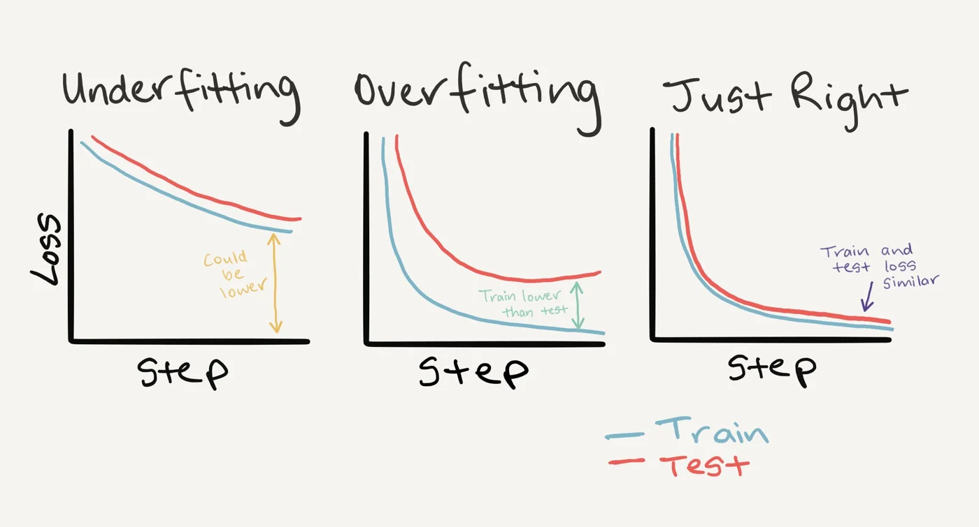 스텝에 따른 학습 손실(파랑)과 테스트 손실(빨강). 왼쪽(Underfitting)은 두 곡선이 천천히 내려가지만 여전히 높아 “더 낮아질 수 있는” 상태, 가운데(Overfitting)는 학습 손실이 테스트 손실보다 훨씬 낮은 상태, 오른쪽(Just Right)은 두 곡선이 빠르게 내려가 비슷한 값에서 만나는 상태다. 출처: learnpytorch.io (Daniel Bourke, MIT License).
가운데 그림에서 테스트 손실(빨강)은 초반에 내려가다가 오히려 다시 올라가기 시작한다. 학습 손실은 계속 내려가므로 두 곡선 사이의 간격이 벌어진다. 이 간격이 과적합의 신호다. 손실 곡선의 다른 모양들은 Google의 Interpreting Loss Curves 가이드에 정리되어 있다.
과적합 다루기
과적합은 모델이 학습 데이터에 너무 잘 맞는 것이므로 “고삐를 죄는” 기법을 쓴다. 이런 기법을 통틀어 정규화(regularization) 라 한다.
| 방법 | 내용 |
|---|---|
| 데이터 더 모으기 | 데이터가 많을수록 새 예시에 일반화되는 패턴을 배울 기회가 많다 |
| 모델 단순화 | 층 수나 층당 은닉 유닛 수를 줄여 지나치게 복잡한 모델을 단순하게 만든다 |
| 데이터 증강 | 학습 데이터에 인위적인 다양성을 더해 학습을 어렵게 만든다. 증강된 데이터에서 패턴을 배운 모델은 더 잘 일반화할 수 있다 |
| 전이 학습(transfer learning) | 다른 모델이 학습한 패턴(사전 학습 가중치)을 내 작업의 출발점으로 쓴다 |
| 드롭아웃 층 | 은닉층 사이의 연결을 무작위로 제거해 모델을 단순화하고 남은 연결을 강하게 만든다(torch.nn.Dropout()) |
| 학습률 감쇠(learning rate decay) | 학습이 진행될수록 학습률을 줄인다. 소파 뒤의 동전을 집을 때 가까워질수록 손을 작게 움직이는 것과 같다 |
| 조기 종료(early stopping) | 과적합이 시작되기 전에 학습을 멈추고, 예컨대 최근 10 에폭 동안 손실이 줄지 않으면 손실이 가장 낮았던 시점의 가중치를 쓴다 |
딥러닝은 데이터의 패턴을 너무 잘 배우기 때문에, 과적합은 딥러닝의 주된 문제 중 하나다.
과소적합 다루기
과소적합 모델은 학습 세트와 테스트 세트 모두에서 예측력이 낮다. 현재의 model_0가 과소적합 상태다. 핵심은 모델의 예측력을 높이는 것이다.
| 방법 | 내용 |
|---|---|
| 층이나 유닛 늘리기 | 은닉층 수나 층당 유닛 수를 늘려 필요한 패턴을 배울 능력을 키운다 |
| 학습률 조정 | 학습률이 너무 커서 매번 가중치를 지나치게 바꾸느라 아무것도 배우지 못할 수 있다. 학습률을 낮춰 본다 |
| 전이 학습 | 이미 잘 작동하는 모델의 패턴을 가져와 내 문제에 맞게 조정한다. 과적합과 과소적합 모두에 도움이 된다 |
| 더 오래 학습하기 | 표현을 배우는 데 시간이 더 필요할 수 있다 |
| 정규화 줄이기 | 과적합을 너무 막으려다 과소적합이 될 수 있으므로 정규화 기법을 덜 쓴다 |
둘 사이의 균형
위 방법 중 어느 것도 만능은 아니다. 한쪽을 지나치게 막으면 다른 쪽이 생길 수 있어서, 과적합과 과소적합 사이의 균형은 머신러닝에서 가장 활발한 연구 분야 중 하나다. 둘 모두에 가장 강력한 기법은 아마 전이 학습일 것이다. 비슷한 문제에서 이미 잘 작동하는 모델(paperswithcode.com/sota나 Hugging Face models 등)을 가져와 내 데이터에 적용한다.
Model 1: 데이터 증강을 쓴 TinyVGG
이번에는 학습 데이터에 TrivialAugmentWide를 적용한다. 모델과 나머지 설정은 그대로 두고 학습 DataLoader만 바꾼다.
# 학습용: 증강 포함
train_transform_trivial_augment = transforms.Compose([
    transforms.Resize((64, 64)),
    transforms.TrivialAugmentWide(num_magnitude_bins=31),
    transforms.ToTensor()
])

# 테스트용: 증강 없음
test_transform = transforms.Compose([
    transforms.Resize((64, 64)),
    transforms.ToTensor()
])

train_data_augmented = datasets.ImageFolder(train_dir, transform=train_transform_trivial_augment)
test_data_simple = datasets.ImageFolder(test_dir, transform=test_transform)

torch.manual_seed(42)
train_dataloader_augmented = DataLoader(train_data_augmented, batch_size=BATCH_SIZE,
                                        shuffle=True, num_workers=NUM_WORKERS)
test_dataloader_simple = DataLoader(test_data_simple, batch_size=BATCH_SIZE,
                                    shuffle=False, num_workers=NUM_WORKERS)
증강은 DataLoader가 이미지를 꺼낼 때마다 무작위로 적용되므로, 같은 이미지도 에폭마다 다른 모습으로 모델에 들어간다. 데이터 파일 수는 225장 그대로다.
torch.manual_seed(42)
torch.cuda.manual_seed(42)

model_1 = TinyVGG(input_shape=3, hidden_units=10,
                  output_shape=len(train_data_augmented.classes)).to(device)

loss_fn = nn.CrossEntropyLoss()
optimizer = torch.optim.Adam(params=model_1.parameters(), lr=0.001)

start_time = timer()
model_1_results = train(model=model_1,
                        train_dataloader=train_dataloader_augmented,  # 유일하게 바뀐 부분
                        test_dataloader=test_dataloader_simple,
                        optimizer=optimizer,
                        loss_fn=loss_fn,
                        epochs=NUM_EPOCHS)
end_time = timer()
print(f"Total training time: {end_time-start_time:.3f} seconds")
Epoch: 1 | train_loss: 1.1074 | train_acc: 0.2500 | test_loss: 1.1058 | test_acc: 0.2604
Epoch: 2 | train_loss: 1.0791 | train_acc: 0.4258 | test_loss: 1.1382 | test_acc: 0.2604
Epoch: 3 | train_loss: 1.0803 | train_acc: 0.4258 | test_loss: 1.1685 | test_acc: 0.2604
Epoch: 4 | train_loss: 1.1285 | train_acc: 0.3047 | test_loss: 1.1623 | test_acc: 0.2604
Epoch: 5 | train_loss: 1.0880 | train_acc: 0.4258 | test_loss: 1.1472 | test_acc: 0.2604
Total training time: 4.924 seconds
Model 1의 손실 곡선
plot_loss_curves(model_1_results)
이번에도 곡선이 좋지 않다. 과소적합인지, 과적합인지, 둘 다인지 생각해 볼 만하다. 이미 과소적합 상태인 모델에 학습을 더 어렵게 만드는 증강(정규화의 일종)을 더했으니 나아지지 않는 것이 자연스럽다. 목표는 정확도를 높이고 손실을 낮추는 것이므로, 위 표의 과소적합 대응책(더 큰 모델, 더 긴 학습, 더 많은 데이터, 전이 학습)이 다음 후보다.
모델 결과 비교
두 모델 모두 성능이 나쁘지만, 비교하는 코드를 작성해 둔다. 결과 사전을 pandas DataFrame으로 바꾼다.
import pandas as pd
model_0_df = pd.DataFrame(model_0_results)
model_1_df = pd.DataFrame(model_1_results)
model_0_df
   train_loss  train_acc  test_loss  test_acc
0    1.107833   0.257812   1.136041  0.260417
1    1.084713   0.425781   1.162014  0.197917
2    1.115697   0.292969   1.169704  0.197917
3    1.095564   0.414062   1.138373  0.197917
4    1.098520   0.292969   1.142631  0.197917
네 지표를 2×2 격자에 두 모델씩 겹쳐 그린다.
plt.figure(figsize=(15, 10))
epochs = range(len(model_0_df))

for i, (col, title) in enumerate([("train_loss", "Train Loss"), ("test_loss", "Test Loss"),
                                  ("train_acc", "Train Accuracy"), ("test_acc", "Test Accuracy")]):
    plt.subplot(2, 2, i + 1)
    plt.plot(epochs, model_0_df[col], label="Model 0")
    plt.plot(epochs, model_1_df[col], label="Model 1")
    plt.title(title)
    plt.xlabel("Epochs")
    plt.legend()
두 모델 모두 비슷하게 나쁘고, 지표가 에폭마다 크게 오르내린다. model_2를 만든다면 무엇을 바꿀지(유닛 수, 에폭 수, 데이터 양, 전이 학습)가 다음 실험의 출발점이다.
직접 고른 이미지로 예측하기
학습한 모델로 데이터셋 밖의 내 이미지를 예측하려면, 그 이미지를 모델이 학습한 데이터와 같은 형식으로 전처리해야 한다. 강의 저장소에서 피자 사진 한 장을 내려받는다.
import requests

custom_image_path = data_path / "04-pizza-dad.jpeg"

if not custom_image_path.is_file():
    with open(custom_image_path, "wb") as f:
        # GitHub에서 내려받을 때는 "raw" 링크를 써야 한다
        request = requests.get("https://raw.githubusercontent.com/mrdbourke/pytorch-deep-learning/main/images/04-pizza-dad.jpeg")
        print(f"Downloading {custom_image_path}...")
        f.write(request.content)
else:
    print(f"{custom_image_path} already exists, skipping download.")
이미지를 텐서로 읽기
torchvision.io.read_image()는 JPEG이나 PNG를 읽어 uint8 자료형, [0, 255] 범위의 3차원 텐서로 돌려준다.
import torchvision

custom_image_uint8 = torchvision.io.read_image(str(custom_image_path))
print(f"Custom image shape: {custom_image_uint8.shape}")
print(f"Custom image dtype: {custom_image_uint8.dtype}")
Custom image shape: torch.Size([3, 4032, 3024])
Custom image dtype: torch.uint8
모델은 [0, 1] 범위의 torch.float32 텐서로 학습했으므로 그대로 넣으면 오류가 난다.
RuntimeError: Input type (torch.cuda.ByteTensor) and weight type (torch.cuda.FloatTensor) should be the same
자료형을 float32로 바꾸고 255로 나눠 범위를 맞춘다.
custom_image = torchvision.io.read_image(str(custom_image_path)).type(torch.float32)
custom_image = custom_image / 255.   # [0, 255] -> [0, 1]

print(f"Custom image shape: {custom_image.shape}")
print(f"Custom image dtype: {custom_image.dtype}")
Custom image shape: torch.Size([3, 4032, 3024])
Custom image dtype: torch.float32
학습된 모델로 예측하기
남은 차이는 모양이다. 모델은 [3, 64, 64]로 학습했는데 이 이미지는 [3, 4032, 3024]다. matplotlib으로 확인할 때는 custom_image.permute(1, 2, 0)으로 HWC로 바꾼다. 크기는 transforms.Resize()로 맞춘다.
custom_image_transform = transforms.Compose([
    transforms.Resize((64, 64)),
])
custom_image_transformed = custom_image_transform(custom_image)

print(f"Original shape: {custom_image.shape}")
print(f"New shape: {custom_image_transformed.shape}")
Original shape: torch.Size([3, 4032, 3024])
New shape: torch.Size([3, 64, 64])
이대로 model_1(custom_image_transformed)를 부르면 장치 오류가 난다.
RuntimeError: Expected all tensors to be on the same device, but found at least two devices, cpu and cuda:0!
.to(device)를 붙여도 이번에는 모양 오류가 난다. 모델은 앞에 배치 차원이 있는 NCHW를 기대하는데 이미지는 CHW이기 때문이다. unsqueeze(dim=0)로 배치 크기 1을 붙인다.
model_1.eval()
with torch.inference_mode():
    custom_image_transformed_with_batch_size = custom_image_transformed.unsqueeze(dim=0)
    print(f"Custom image transformed shape: {custom_image_transformed.shape}")
    print(f"Unsqueezed custom image shape: {custom_image_transformed_with_batch_size.shape}")

    custom_image_pred = model_1(custom_image_transformed.unsqueeze(dim=0).to(device))
Custom image transformed shape: torch.Size([3, 64, 64])
Unsqueezed custom image shape: torch.Size([1, 3, 64, 64])
방금 겪은 것이 딥러닝과 PyTorch에서 가장 흔한 세 가지 오류다.
- 자료형이 틀림: 모델은
torch.float32를 기대하는데 이미지는uint8이었다. - 장치가 틀림: 모델은 GPU에 있는데 데이터는 아직 CPU에 있었다.
- 모양이 틀림: 모델은
[N, C, H, W]를 기대하는데 이미지는[C, H, W]였다.
이 오류들은 사용자 이미지에만 생기는 것이 아니라 텍스트, 오디오, 정형 데이터 등 거의 모든 데이터와 문제에서 나타난다.
예측은 아직 로짓이므로 로짓 -> 예측 확률 -> 예측 레이블로 바꾸고, 레이블 인덱스로 클래스 이름을 찾는다.
class_names = train_data_simple.classes

custom_image_pred_probs = torch.softmax(custom_image_pred, dim=1)
custom_image_pred_label = torch.argmax(custom_image_pred_probs, dim=1)
print(f"Prediction logits: {custom_image_pred}")
print(f"Prediction probabilities: {custom_image_pred_probs}")
print(f"Prediction label: {custom_image_pred_label}")

custom_image_pred_class = class_names[custom_image_pred_label.cpu()]  # 인덱싱 전에 CPU로
custom_image_pred_class
Prediction logits: tensor([[ 0.1172,  0.0160, -0.1425]], device='cuda:0')
Prediction probabilities: tensor([[0.3738, 0.3378, 0.2883]], device='cuda:0')
Prediction label: tensor([0], device='cuda:0')
'pizza'
평가 지표는 나빴는데도 “pizza”를 맞혔다. 하지만 세 클래스의 확률이 거의 같다(0.37, 0.34, 0.29). 이렇게 비슷한 확률은 (1) 이미지에 세 음식이 모두 있어서 모델이 세 클래스를 동시에 예측하려 하거나, (2) 모델이 무엇을 예측할지 몰라 비슷한 값을 나눠 주는 경우일 수 있다. 여기서는 모델이 제대로 학습되지 않았으므로 (2), 즉 추측에 가깝다. 또 이 모델은 어떤 이미지를 넣어도 피자, 스테이크, 초밥 중 하나로만 답한다. 다른 클래스를 예측하게 하려면 그 클래스로 학습시켜야 한다.
예측 과정을 함수로 묶기
매번 위 단계를 반복하지 않도록 함수로 만든다.
- 이미지 경로를 받아
torch.float32로 읽는다. - 픽셀 값을
[0, 1]로 나눈다. - 필요하면 변환한다.
- 모델을 대상 장치로 옮긴다.
- 배치 차원을 붙이고 같은 장치에서 예측한다.
- 로짓을 예측 확률로 바꾼다.
- 예측 확률을 예측 레이블로 바꾼다.
- 이미지와 예측, 예측 확률을 함께 그린다.
def pred_and_plot_image(model: torch.nn.Module,
                        image_path: str,
                        class_names: List[str] = None,
                        transform=None,
                        device: torch.device = device):
    """대상 이미지를 예측하고 예측 결과와 함께 그린다."""
    # 1-2
    target_image = torchvision.io.read_image(str(image_path)).type(torch.float32)
    target_image = target_image / 255.

    # 3
    if transform:
        target_image = transform(target_image)

    # 4
    model.to(device)

    # 5
    model.eval()
    with torch.inference_mode():
        target_image = target_image.unsqueeze(dim=0)
        target_image_pred = model(target_image.to(device))

    # 6-7
    target_image_pred_probs = torch.softmax(target_image_pred, dim=1)
    target_image_pred_label = torch.argmax(target_image_pred_probs, dim=1)

    # 8. [1, C, H, W] -> [C, H, W] -> [H, W, C]
    plt.imshow(target_image.squeeze().permute(1, 2, 0))
    if class_names:
        title = f"Pred: {class_names[target_image_pred_label.cpu()]} | Prob: {target_image_pred_probs.max().cpu():.3f}"
    else:
        title = f"Pred: {target_image_pred_label} | Prob: {target_image_pred_probs.max().cpu():.3f}"
    plt.title(title)
    plt.axis(False)

pred_and_plot_image(model=model_1,
                    image_path=custom_image_path,
                    class_names=class_names,
                    transform=custom_image_transform,
                    device=device)
제목에 “Pred: pizza”와 최대 확률이 표시된다. 이번에는 추측으로 맞혔지만 다른 이미지에서는 그렇지 않을 수 있다. 64×64로 줄였기 때문에 그림도 뭉개져 보인다.
정리
- 데이터 증강은 학습 데이터의 다양성을 인위적으로 늘려 일반화를 돕는다.
transforms.TrivialAugmentWide(num_magnitude_bins=31)는 무작위 변환을 무작위 강도로 적용하며, 증강은 학습 세트에만 한다. - TinyVGG를 컬러 64×64 이미지에 맞게
in_channels=3,in_features=10*16*16으로 만들고, 이미지 한 장으로 순전파를 시험한 뒤torchinfo.summary()로 층별 모양과 매개변수 수(10,693개)를 확인했다. train_step(),test_step(),train()으로 학습을 함수화하고, 에폭별train_loss,train_acc,test_loss,test_acc를 사전에 모아 손실 곡선을 그렸다.- 학습 손실이 테스트 손실보다 훨씬 낮으면 과적합, 둘 다 높으면 과소적합이며, 이상적인 곡선은 낮은 곳에서 서로 겹친다.
- 과적합에는 데이터 추가, 모델 단순화, 증강, 전이 학습, 드롭아웃, 학습률 감쇠, 조기 종료를, 과소적합에는 모델 키우기, 학습률 조정, 전이 학습, 더 긴 학습, 정규화 줄이기를 쓴다.
- 225장으로 5 에폭 학습한 두 모델은 증강 여부와 관계없이 무작위 추측 수준(손실 약 1.10)이었다. 과소적합 모델에 증강을 더하는 것만으로는 나아지지 않았다.
- 내 이미지를 예측할 때는 세 가지 흔한 오류, 즉 자료형(
uint8→float32와/255), 장치(.to(device)), 모양(Resize와unsqueeze(dim=0))을 모두 맞춰야 한다.